
Every enterprise data platform eventually hits the same wall. Analytical data exists in two places: a data lake (cheap, scalable, ungoverned) and a data warehouse (expensive, fast, governed). Between them sits an ETL pipeline that copies, transforms, and reconciles — creating a permanent tax on engineering time, data freshness, and infrastructure spend.
The symptoms are familiar. Dashboards show yesterday's numbers because the warehouse loads overnight. ML models train on stale copies because the warehouse does not support Python-native access. Storage bills grow because the same curated datasets live in both systems simultaneously. Governance fragments because access controls, lineage, and audit trails cannot span two architecturally different platforms.
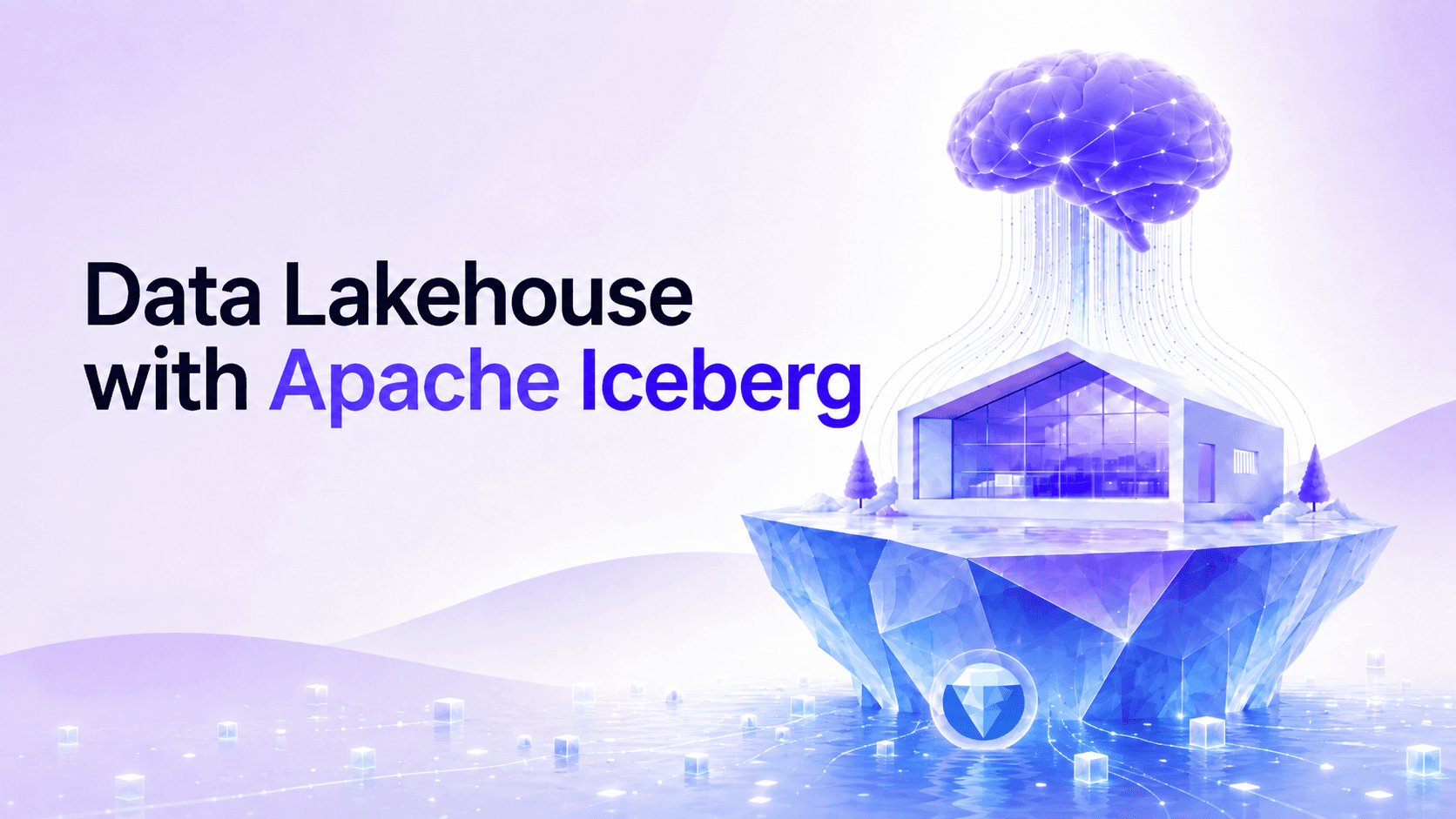
The data lakehouse resolves this by collapsing both systems into one: transactional guarantees applied directly to data on object storage. One copy. One governance model. Any engine — SQL, ML, streaming, AI — reads and writes the same tables with full ACID safety. The warehouse is not replaced by a different product; the lake _becomes_ the warehouse through a metadata innovation called a table format.
The practical result: BI dashboards, Spark ML pipelines, Flink streaming jobs, and autonomous AI agents all query the same governed tables — without ETL between them, without stale copies, without paying warehouse markup on storage that costs $0.023/GB/month in its native form.
This guide explains how a data lakehouse actually works — from storage to compute to catalog to the operational reality that most guides skip. It covers the four architectural layers, how Apache Iceberg's metadata tree enables transactional guarantees, how data flows through the medallion tiers, why every production lakehouse degrades over time, and how an intelligent control plane like LakeOps closes the gap between the architecture you build and the performance you need.
The four layers of a data lakehouse
A data lakehouse is not a monolithic system. It is four cooperating layers — each handling a specific responsibility, each independently evolvable. Understanding how they interact is the foundation for building one that performs in production.
Layer 1: Object storage
All data resides on cloud object storage — S3, GCS, or ADLS. This is where the economics originate. Object storage provides eleven-nines durability at $20–25 per TB per year. A petabyte of analytical data costs roughly $20,000/year to persist — compared to $500,000+ when that same data sits inside a traditional warehouse with bundled compute.
Storage is decoupled from everything above it. Shut down every query engine and the data remains. Add a new engine tomorrow — it reads from the same bucket. Move clouds — the files copy byte-for-byte with no format conversion.
Data lands as Apache Parquet files — a columnar format that stores values by column rather than by row. A query touching 5 columns from a 300-column table physically reads only those 5 columns. Parquet also embeds per-column min/max statistics in each file header, enabling query engines to skip entire files whose value ranges cannot satisfy the WHERE clause. This skip-scanning is what makes lakehouse queries competitive with warehouse queries — but only when files are properly sized and organized.
Layer 2: The table format — Apache Iceberg
A directory of Parquet files on S3 is a data lake — readable, but not transactional. The table format is the metadata innovation that adds the missing guarantees.
Apache Iceberg — the dominant open table format as of 2026, supported natively by Spark, Trino, Flink, DuckDB, Snowflake, Databricks, Athena, and StarRocks — provides ACID commits, schema evolution capabilities, time travel, partition evolution, and concurrent multi-writer safety through a metadata tree architecture. At the Iceberg Summit 2026, the community confirmed that Iceberg has crossed the threshold from adoption to optimization: every major cloud vendor and data platform now reads and writes the format natively, and the focus has shifted to V3 features (deletion vectors, row lineage) and the V4 specification. For a deep dive into the full five-layer stack, see the Iceberg lakehouse architecture guide.
How Iceberg's metadata tree works
Each Iceberg table maintains a hierarchy of metadata files on the same object storage as the data:
- 1.A metadata pointer (tracked by the catalog) — points to the current table version
- 2.Snapshot files — each representing the table's complete state at a point in time. Every write creates a new snapshot.
- 3.Manifest lists — each snapshot references a manifest list that indexes the active manifests
- 4.Manifests — each tracking a batch of data files with per-file statistics (path, partition values, row count, column min/max)
- 5.Data files — the actual Parquet files containing rows
This tree enables two properties that make the lakehouse viable:
Atomic commits. Every write produces new data files and a new snapshot. The catalog atomically swaps the pointer from old snapshot to new. Readers always see a consistent state. Failed writes leave no trace — the pointer was never advanced.
Statistical pruning. Query engines read manifests (kilobytes) to determine which data files (gigabytes) are relevant. A query filtering on country = 'DE' checks manifest-level statistics and skips every file whose country column's min/max range excludes 'DE'. No data read. No I/O wasted. This is why lakehouse queries can match warehouse speed — but only when the metadata is current and the data layout aligns with query patterns.
The critical implication: every commit grows the tree. Every streaming write adds files. Every mutation adds delete markers. The tree that enables fast queries also accumulates entropy that _degrades_ query speed over time — unless something actively maintains it.
Layer 3: The catalog
The catalog is the coordination service that answers: where is the current metadata pointer for each table, and how do multiple engines safely coordinate writes?
Every engine — Spark, Trino, Flink, DuckDB — consults the catalog before each read (to locate current metadata) and during each write (to commit atomically). Without the catalog, concurrent writers could corrupt table state. With it, they race safely: one commits, the other retries against updated state.
Modern lakehouses use the Iceberg REST Catalog specification — a standard HTTP API that every engine implements. Adding a new engine is a configuration change (point it at the catalog URL), not an integration project. Catalog options include managed services (AWS Glue), open-source servers (Apache Polaris, Lakekeeper), federated solutions (Apache Gravitino), and Git-branching models (Project Nessie) — all speaking the same REST protocol.
The catalog is also where access control, retention policies, and audit logging materialize. It is the governance anchor for multi-engine environments where every engine must see consistent permissions.
Layer 4: Compute engines
The lakehouse separates compute from storage, enabling multiple specialized engines to operate on the same data concurrently:
- Spark — batch ETL, ML training, complex multi-stage transformations. The workhorse for heavy writes and joins.
- Trino — interactive SQL with sub-second response times. Excels at dashboard queries and ad-hoc exploration.
- Flink — streaming ingestion with exactly-once semantics. Continuous CDC from operational databases into lakehouse tables.
- DuckDB — embedded analytics for notebooks, CI/CD pipelines, and single-node processing. Zero infrastructure overhead.
- Snowflake / Athena / StarRocks — managed engines for specific workload profiles (high-concurrency BI, serverless ad-hoc, real-time OLAP).
Each engine discovers tables through the same REST catalog and reads/writes through Iceberg's transactional protocol. They coexist safely on the same tables through snapshot isolation. This is the key architectural advantage over the warehouse model: instead of one vendor's engine for everything, you use the best tool for each workload shape.
But multi-engine access multiplies operational pressure. More engines means more write patterns, more file fragmentation profiles, and more divergent query patterns competing for the same table's physical layout — creating the operational challenge that defines production lakehouse management.
How data flows through a production lakehouse
How does data actually move from source systems through the lakehouse to consumers? The medallion architecture (bronze → silver → gold) is the standard pattern for organizing this flow, and each tier creates different operational characteristics that matter for long-term health.
Bronze: the raw capture layer
Source data lands in its original form. CDC events from PostgreSQL captured by Debezium and written by Flink. Clickstream events from Kafka. Daily batch exports from SaaS APIs. Partner file drops. Everything arrives as append-only, schema-on-read, immutable records.
Bronze is the replay source. When silver-layer transformation logic has a bug discovered months later, you rebuild from bronze. When a new use case requires fields that were previously ignored, they are already preserved in bronze. This immutability is non-negotiable — teams that apply transformations at ingestion lose the ability to retrospectively correct logic errors.
What this means operationally: Streaming CDC with 5-minute commits creates approximately 8,600 new files per table per month. A lakehouse ingesting from 20 operational databases at sub-minute latency accumulates hundreds of thousands of files across its bronze layer within weeks. Individual file sizes average 5–20 MB — far below the 256–512 MB target where engines perform optimally. File count — not data volume — is what degrades query planning speed.
Silver: the governed truth layer
Silver transforms bronze into a data model that the organization commits to: one row per entity, resolved foreign keys, deduplicated events, enforced types, quarantined bad records. Silver is not a cleanup step — it is an architectural commitment to a domain model that all downstream consumers depend on.
Key transformations include deduplication (resolving late-arriving records and replay duplicates through MERGE INTO), type enforcement and validation, slowly changing dimensions (SCD Type 2), and reference data enrichment. Each of these generates write patterns with operational implications.
What this means operationally: Silver tables receive MERGE INTO operations — upserts that create delete markers (position-delete files or V3 deletion vectors) that every subsequent read must reconcile. A CDC table receiving 50,000 updates per hour generates thousands of delete markers per day. Without periodic resolution of these markers, query latency creeps 2–5x higher while the table reports the same row count and appears unchanged to basic monitoring.
Gold: the consumer-optimized layer
Gold tables exist for performance: pre-aggregated metrics for dashboards, denormalized feature tables for ML training, materialized snapshots for compliance reporting. Gold trades storage redundancy for read speed.
What this means operationally: Gold tables are typically overwritten on a schedule — daily, hourly, or triggered by upstream freshness signals. Each OVERWRITE operation atomically replaces the table's content but leaves previous snapshots' files in storage until explicitly expired. A daily gold refresh creates 365 snapshots per year. At 50 GB per refresh, that is 18 TB of stale data files persisting in storage — even though only the latest 50 GB is logically current. Without snapshot lifecycle management, storage grows linearly forever from data that was replaced weeks or months ago.
The maintenance gradient
The three tiers create a gradient of operational need:
- Bronze → small-file pressure (compaction priority)
- Silver → delete-file pressure (merge resolution priority)
- Gold → stale-snapshot pressure (expiration priority)
No uniform maintenance schedule handles this correctly. Each table needs the _right_ operation at the _right_ cadence — determined by its ingestion velocity, mutation pattern, and query load. This is the insight that leads directly to the control plane model.
What the lakehouse unlocks
The economic case (10–50x cheaper storage) is straightforward. The architectural case is more powerful: eliminating the boundaries between workload types that the two-system model enforced.
BI and reporting. Dashboards query silver and gold tables directly through Trino or Snowflake. No warehouse sync delay. No overnight ETL window. Time travel lets analysts reproduce the exact state of any report at any prior date — critical for regulated industries. Performance depends on table health: well-compacted tables with accurate column statistics enable engines to prune 90%+ of files on selective queries. When a BI dashboard filters on region = 'EMEA' AND quarter = 'Q2', a properly maintained table skips every file that cannot contain matching rows. A degraded table forces a full scan regardless of how selective the filter is.
ML and feature engineering. ML pipelines read training data from the same governed tables that power dashboards — eliminating training-serving skew, the most common source of ML model degradation in production. Experiment reproducibility comes free: pin to a snapshot ID, retrain on byte-for-byte identical data months later. Feature stores built on lakehouse tables inherit versioning, access control, lineage, and time travel from the table format.
Streaming analytics. Flink and Spark Structured Streaming write directly to lakehouse tables with exactly-once transactional guarantees. The same transformation logic runs as streaming (for freshness) or batch (for cost) by changing only the trigger configuration. This eliminates the lambda architecture's core problem: maintaining two parallel pipelines with identical logic that inevitably drift apart.
AI agents as first-class consumers. In 2026, AI agents autonomously discover schemas, formulate queries, and feed results into multi-step reasoning chains. The lakehouse is their knowledge infrastructure — providing structured, governed, queryable data that agents access through standard protocols like MCP. Agent workloads differ from human workloads in ways that compound at scale: unpredictable query patterns that no static sort order can pre-optimize for, high concurrency that creates pressure on table health, cost sensitivity where slow queries burn token budgets on waiting, and no self-diagnosis when queries slow down because the table needs compaction. For a comprehensive guide to making your lakehouse AI-ready, see the pillar article.
Why every production lakehouse degrades
Here is what most lakehouse guides skip entirely. The four layers give you the architecture. They do not give you a system that _stays healthy_. Every production lakehouse — without exception — degrades over time unless something actively maintains it. This is not a flaw; it is a fundamental consequence of how append-only transactional systems work.
The mechanics of degradation
Iceberg never modifies files in place. Every write creates new files. Every snapshot preserves a complete view. This is what provides transactional safety — but it means the system accumulates structural debt continuously:
File fragmentation. Each commit adds files. Streaming ingestion at 5-minute intervals creates ~8,600 files per table per month, each averaging 12 MB — well below the 256–512 MB target where query engines perform optimally. The engine must open, plan, and coordinate reads across 100x more files than necessary.
Planning overhead. Engine query planners traverse the manifest tree to identify relevant files. At 1,000 files, planning takes milliseconds. At 50,000 files, planning takes 10–20 seconds — sometimes exceeding the query execution itself. The metadata hierarchy that enables fast pruning becomes a bottleneck when it indexes too many undersized files.
Delete-file accumulation. Every UPDATE and DELETE writes markers that subsequent readers must reconcile against data files at read time. A heavily-mutated table accumulates thousands of delete markers. Query latency increases 2–5x while the table's row count and size appear unchanged — making degradation invisible to basic monitoring.
Storage waste. Expired logical content leaves physical files behind. Orphaned files from failed writes, aborted compaction, and expired snapshots accumulate in storage. Without active cleanup, production lakehouses accumulate terabytes of unreferenced files — pure cost with no analytical value.
Compounding pressure. These forces are not independent — they compound. More files means larger manifests. Larger manifests means slower planning. Slower planning means longer maintenance operations. Longer maintenance operations means less frequent runs. Less frequent runs means more file accumulation. The system has a natural tendency toward runaway degradation that accelerates once it begins.
Why manual maintenance does not scale
The instinct is to write scripts: a Spark job that compacts every table nightly, a cron that expires old snapshots weekly. This works for 5–10 tables. It fails at production scale for structural reasons:
Tables need different cadences. A streaming table needs compaction hourly. A daily-refresh table needs it weekly. A slowly-growing dimension needs it monthly. One schedule cannot serve all three without either wasting compute on healthy tables or neglecting degraded ones.
Operations have dependencies. Compacting files that will be expired next hour is wasted work. Rewriting manifests before compaction invalidates the rewrite. The five maintenance operations must run in a specific sequence — and re-sequence when conditions change.
Static thresholds drift. 'Compact when file count exceeds 1,000' is reasonable for one table's current state. But partition cardinality changes, ingestion velocity shifts, query patterns evolve. The threshold that was correct last month is wrong today — and nobody adjusts it until the table is already degraded.
Execution cost. Running Spark clusters for file-rewrite operations costs ~$50/TB in compute — making continuous maintenance prohibitively expensive. Teams are forced into overnight-only windows where tables degrade for 23 hours between passes.
The control plane: closing the operational gap
The answer is not better scripts or more sophisticated cron. It is an architecturally different approach: a control plane that operates the lakehouse as a closed-loop system — continuously sensing table state, reasoning about what each table needs, executing the right operations in the right sequence, and learning from outcomes to improve future decisions.
The concept comes from distributed systems. In Kubernetes, the control plane observes cluster state and reconciles toward desired state — without replacing the containers or VMs underneath. Applied to a lakehouse: the control plane observes table health across every catalog and engine, decides what maintenance each table needs, executes it in the correct sequence, and learns from outcomes. It does not replace your catalog, engines, or storage. It adds the missing operational intelligence layer.
LakeOps is a purpose-built control plane for Apache Iceberg lakehouses. It connects to your existing catalogs and engines through standard APIs and operates without moving data, changing pipelines, or introducing vendor lock-in. Whether you are exploring how lakehouses compare to lakes and warehouses or already operating at scale, the control plane closes the gap between architecture and production performance.
Sense: structural telemetry
The control plane continuously reads metadata from every connected catalog — file counts per partition, file size distributions, manifest depth, snapshot velocity, delete-file ratios, partition-level skew, and cross-engine query patterns. This is metadata inspection, not data access — the control plane never reads or moves your actual data.
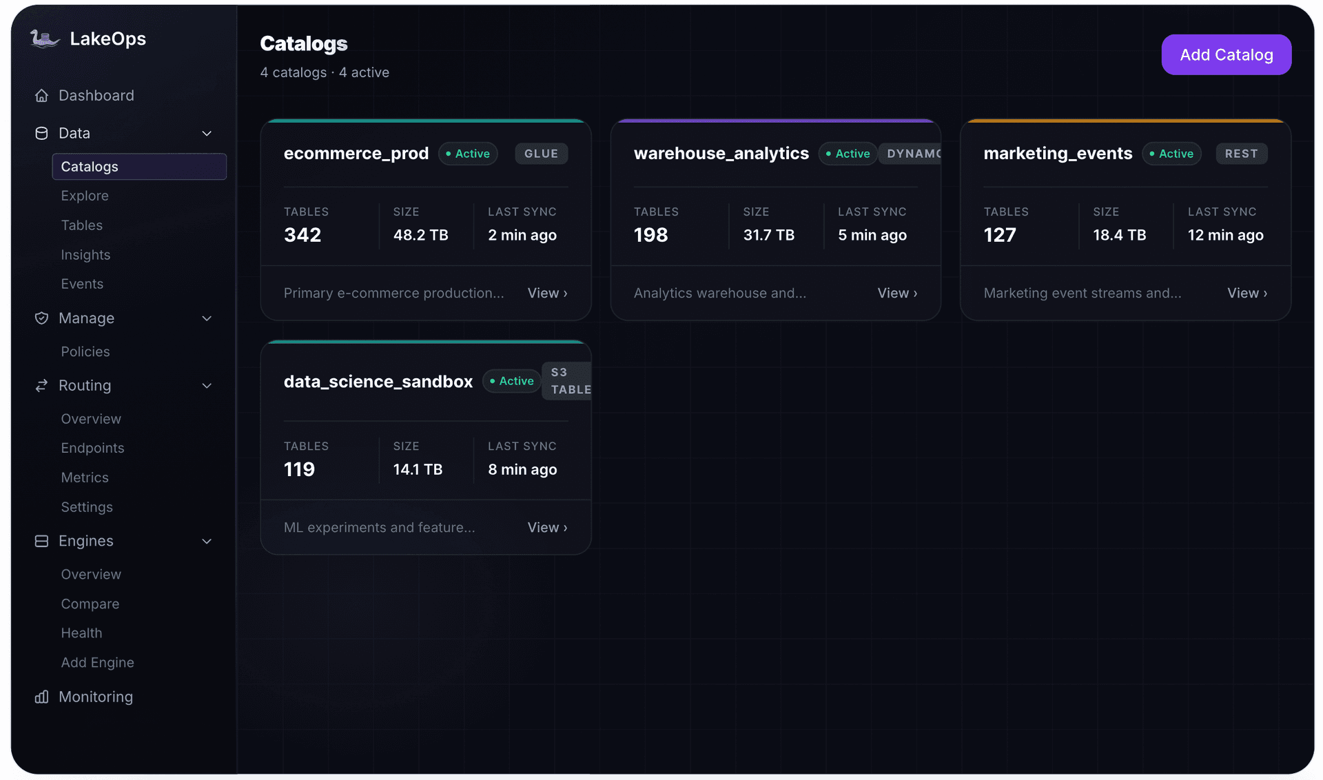
The sensing is passive and lightweight — it adds no load to production engines. It works across any combination of catalogs and engines, aggregating a unified view of table health that no single component in the stack can provide alone.
Assess: health classification
Raw telemetry becomes actionable through health scoring. Every table is continuously classified as Healthy, Warning, or Critical — based on file sizes within target, manifest compactness, delete ratios, sort order alignment with query patterns, and more.

The thresholds are not static defaults. They account for each table's partition cardinality, ingestion velocity, engine mix, and historical maintenance response — adapting automatically as workloads evolve.


LakeOps observability surfaces this classification as a lake-wide dashboard with drill-down into specific metrics, proactive insights at severity levels, and cross-engine telemetry that reveals optimization opportunities no single engine can see.
Plan: sequenced maintenance
For each table classified as Warning or Critical, the control plane determines which operations to run and in what order. The sequencing follows a dependency chain where each step's output becomes the next step's input:
Step 1 → Expire snapshots. Remove snapshots beyond the retention policy. This dereferences files that are no longer needed — reducing the scope for subsequent operations. Step 2 → Remove orphan files. Delete unreferenced files older than the safety window. This captures files newly dereferenced by expiration plus accumulated waste from failed writes. Step 3 → Compact data files. Merge small files into optimally-sized ones. Resolve delete markers so subsequent reads skip reconciliation overhead. Optionally sort data by query-relevant columns to enable statistical pruning. Step 4 → Rewrite manifests. Consolidate the manifest tree to reflect the new compacted layout. Step 5 → Compute statistics. Refresh Puffin column statistics on the compacted files for accurate pruning decisions.

LakeOps managed maintenance runs this pipeline as a coordinated sequence per table — respecting dependencies, avoiding conflicts with active writers, and targeting only the partitions that need work.
Execute: intelligent, continuous optimization
The control plane does not just decide what to run — it executes every operation itself, on a purpose-built engine designed for continuous table maintenance. Most teams run compaction on Spark, but Spark is a general-purpose distributed engine — JVM overhead, GC pauses, OOM risk, cluster provisioning delay. Compaction is a narrow, I/O-bound read-merge-write operation. It does not need a distributed compute framework. It needs a fast, bounded-memory binary that runs continuously in the background.
LakeOps compaction runs on a dedicated Rust engine powered by Apache DataFusion. The engine is fast enough — 200 GB in 221 seconds, 95% faster than Spark — that tables never accumulate enough structural debt to degrade between cycles. And at sub-$5 per TB, it is economical enough to run continuously rather than in overnight windows. The result: maintenance becomes a background process rather than a scheduled event. Tables stay healthy because the control plane acts before degradation begins, not after users complain.
The engine is conflict-aware — it knows which partitions have active writers and excludes them, retries on OCC conflicts automatically, and never expires snapshots that active readers depend on. No coordination scripts needed.
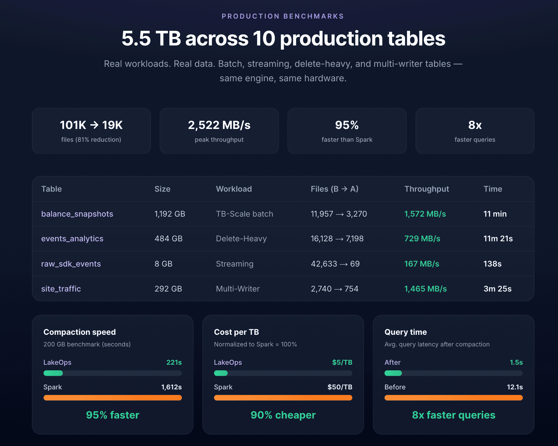
Query-driven sort optimization
Standard compaction merges small files into bigger ones — that helps, but it is only half the optimization. The real leverage comes from sorting data by the columns that production queries actually filter on.
When data within each file spans a narrow value range for the sort columns, statistical pruning becomes surgical: the engine checks file-level min/max metadata and eliminates 90%+ of files before reading any data. The difference between an unsorted table and a properly sorted table is typically 8–12x in query speed.
The control plane learns which columns matter by aggregating WHERE, JOIN, and GROUP BY telemetry from every connected engine — Trino, Spark, Snowflake, Athena, DuckDB. No single engine has the full picture. A table that Trino queries on customer_id and Spark queries on event_date needs a sort order that serves both. The control plane computes this automatically and updates it as patterns shift — when a new dashboard deploys or an AI agent fleet starts querying on different columns.
Before committing any sort strategy to production, the control plane runs layout simulations on Iceberg branches — replaying actual query patterns against the proposed layout and measuring projected scan reduction. Bad sort decisions are caught before they touch production data.

Learn: outcome-driven improvement
After each maintenance cycle, the control plane measures outcomes against expectations. Did file count reach the target? Did planning latency improve? Did the health score advance? Results feed back into the assessment model — tables that responded well to sort compaction on specific columns get those columns reinforced in future cycles. Tables with unusual characteristics get customized strategies without manual configuration.

Over time, this learning loop makes the control plane more precise. Tables with unusual characteristics — very high partition cardinality, extremely bursty ingestion, mixed engine access — get customized strategies automatically, without manual threshold tuning.
Governance: policies that run themselves
Visibility without enforcement is just monitoring. The control plane turns observability into automated governance through declarative policies that operate at multiple scopes:
- Organization-wide defaults — baseline compaction targets, snapshot retention, orphan cleanup schedules applied to every table unless overridden
- Namespace-level rules — production namespaces get aggressive maintenance; staging gets relaxed thresholds
- Per-table exceptions — compliance tables with 365-day retention; hot tables with 15-minute compaction cadence
Policies inherit downward: new tables automatically receive the governance rules of their namespace. No manual configuration per table. No tables falling through the cracks because someone forgot to add them to the maintenance script.

Every policy execution is logged with full audit trail — what ran, when, what changed, duration, bytes before/after.

Query routing: making multi-engine rational
Having multiple engines on the same data is architecturally elegant. But without routing intelligence, it becomes accidentally expensive: queries dispatched to the wrong engine pay the wrong pricing model and get the wrong performance profile.
A point lookup for 100 rows dispatched to Spark burns 30 seconds of cluster startup. That same query on DuckDB resolves in 0.3 seconds. A dashboard query running on Snowflake at $2/credit is 10x more expensive than the same query on a self-hosted Trino cluster. A full-table scan on DuckDB crashes; on Spark, it completes in minutes.
LakeOps query routing provides a single SQL endpoint that dispatches queries to the optimal engine based on workload type, table health state, and cost/latency targets. Define routing groups — analytics, BI, ETL, reports — each mapping to a stable SQL endpoint with engine-specific optimization strategies.
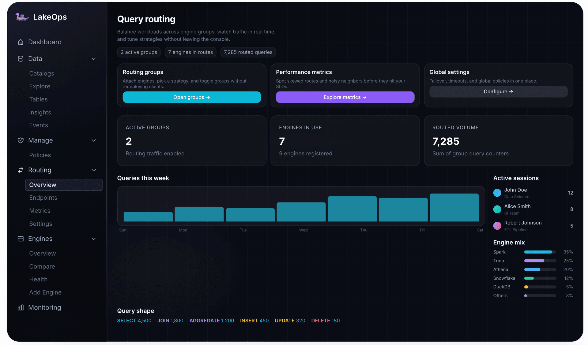

The routing layer and the maintenance layer form a reinforcing loop: as the control plane compacts and sorts tables, more engines become eligible per query shape. More routing options mean lower per-query cost. Lower cost justifies more frequent querying. More querying generates better telemetry for compaction decisions.
AI agent enablement
AI agents cannot diagnose a slow query caused by table degradation. They cannot distinguish 'this data does not exist' from 'this query is slow because the table needs compaction.' When an agent hits a degraded table, it retries, times out, or hallucinates — degrading answer quality without surfacing the root cause. The infrastructure must be healthy _before_ agents query it, not corrected after they fail.
LakeOps provides an MCP-native interface with PostgreSQL, MySQL, and Arrow Flight wire compatibility. Any MCP-compatible agent discovers catalogs, browses schemas, executes queries, and receives results — without custom integration per agent framework.
Layered guardrails enforce per-session constraints: ReadOnly mode blocks DDL and DML. ScanBudget rejects queries whose estimated scan exceeds configurable thresholds. PIIMask hashes sensitive columns before results reach the model. HumanApproval pauses high-stakes operations for review. Guardrails are configured once at the control plane level and enforced uniformly across all agent connections — regardless of which agent framework, which engine, or which table is accessed. For a deep dive into safe AI agent access to Apache Iceberg in production, see the access control guide.
Agent query telemetry feeds back into compaction priorities and routing weights — creating a flywheel where the lake gets smarter as agents use it. Tables that agents query heavily get maintenance priority; sort orders adapt to agent patterns; routing weights shift as agent workloads evolve.
The economic model
The lakehouse's cost advantage operates at four levels that compound:
Storage decoupling. Object storage at $20–25/TB/year vs. warehouse storage at $500–2,000/TB/year. For 200 TB of curated data: $4,000–5,000/year vs. $100,000–400,000/year. At petabyte scale, the savings fund entire platform teams.
Elimination of duplication. The lake-to-warehouse ETL that copies, transforms, and reconciles data disappears — eliminating the compute cost of the ETL pipeline itself, the engineering hours maintaining it, the storage cost of the warehouse copy, and the reconciliation overhead when copies drift.
Multi-engine routing efficiency. When every query runs on the cheapest engine that meets its latency requirement, aggregate compute cost drops dramatically. Without routing, organizations default to Snowflake pricing for everything — $2+ per credit regardless of query complexity.
Maintenance economics. The control plane's Rust-based engine compacts at sub-$5/TB — roughly 90% cheaper than Spark maintenance clusters. This makes _continuous_ maintenance economically viable rather than forcing overnight-only windows where tables degrade for 23 hours between passes.
Combined, organizations operating at 500+ TB report 3–5x total cost reduction compared to warehouse-plus-lake architectures — combining storage savings, duplication elimination, routing-driven compute efficiency, and cheaper maintenance.
Implementing: the practical sequence
You do not need the full architecture on day one. Each step delivers independent value and sets up the next:
1. Start with Iceberg. Choose Apache Iceberg for all new analytical tables. The ecosystem support is universal — every major engine reads and writes it natively. Existing Delta Lake tables interoperate through UniForm.
2. Deploy a REST catalog. This is the coordination point — get it right early. AWS Glue for managed simplicity. Self-hosted Polaris for full control. Gravitino if you need to federate across existing catalogs.
3. Build the ingestion layer (bronze). CDC from operational databases via Flink. Event streams from application telemetry. Batch loads from external sources. Keep it append-only and immutable.
4. Build the semantic layer (silver). Domain modeling, deduplication, quality enforcement. This becomes the organization's governed truth — every downstream consumer starts here.
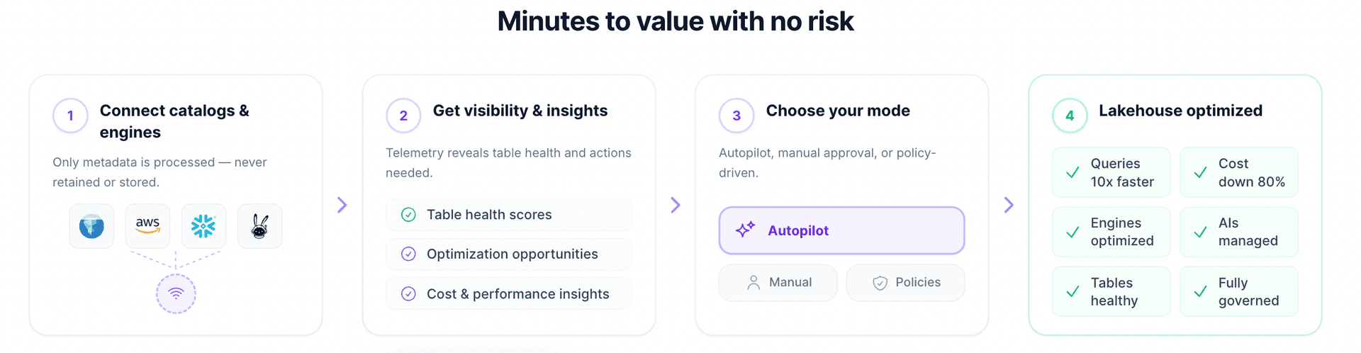
5. Connect the control plane. Once data flows and tables accumulate, connect LakeOps to your catalog. Ten minutes, no data movement, no infrastructure changes. Instant visibility into every table's health state. Start in manual-approval mode — review what the control plane recommends before enabling autonomous execution. Then enable autopilot and let the closed loop run.
6. Add specialized engines. As workloads diversify, add Trino for interactive SQL, DuckDB for notebooks, Snowflake for governed BI access. The REST catalog makes each addition a configuration step.
7. Enable routing and agent access. With 3+ engines, define routing groups. Let the control plane dispatch each query to the optimal backend. Expose tables to agents via MCP with guardrails per agent type. Agent telemetry feeds back into optimization priorities — tables adapt to agent workloads automatically.
Comparing the options
| Characteristic | Data lake | Data warehouse | Data lakehouse |
|---|---|---|---|
| Storage model | Open files on object storage | Proprietary format, vendor storage | Open files on object storage |
| Transactions | None | Full ACID | Full ACID (table format) |
| Governance | Manual, fragmented | Vendor-managed, centralized | Catalog-unified, multi-engine |
| Query speed | Depends entirely on maintenance | Vendor-optimized, consistent | Matches warehouse when maintained |
| Engine flexibility | Any tool reads files | Vendor's engine only | Multiple engines, REST catalog |
| ML/AI workloads | Native but ungoverned | Export required | Native and governed |
| Streaming | Separate infrastructure | Separate infrastructure | Same tables, same transactions |
| Cost at petabyte | ~$20K/yr storage | ~$500K+/yr storage+compute | ~$20K/yr storage + operations |
| Maintenance burden | None (no transactions) | Zero (vendor manages) | Requires control plane |
| Vendor lock-in | Low | High | Low (open formats + catalog) |
To understand where each architecture fits, see how Iceberg compares to Delta Lake for a format-level comparison.
The lakehouse occupies a specific position: warehouse guarantees at lake economics, with the trade-off that operational maintenance is your responsibility rather than a vendor's. The control plane is what makes this trade-off viable at scale — providing vendor-grade operational ease without the vendor lock-in.
When to build a data lakehouse
Not every team needs this architecture. A single-engine, single-workload team at moderate scale gets reasonable value from a managed warehouse without the operational complexity. But the lakehouse becomes the correct choice when:
- Multiple workload types coexist. BI, ML, streaming, and AI workloads need the same data with different access patterns and different engines.
- Scale makes economics matter. Above 50–100 TB of analytical data, the storage cost differential (10–50x) becomes significant enough to fund an entire platform team.
- Multi-engine is a requirement. Different teams genuinely need different engines — Spark for ETL, Trino for interactive, Flink for streaming, DuckDB for development.
- Vendor independence is a priority. Open formats on your own storage mean no single vendor controls your exit path. Every component decision is reversible.
- AI/ML is a first-class workload. Models and agents need native, governed access to analytical data — not exports, not API wrappers, not stale copies in separate feature stores.
If three or more of these apply, the lakehouse is not a future consideration — it is the architecture to build toward now.
Conclusion
The data lakehouse is the production standard for teams that need BI, ML, streaming, and AI on the same governed data without warehouse pricing or lake-quality compromises.
Building one is an assembly problem: object storage for economics, Apache Iceberg for transactional guarantees, a REST catalog for coordination, and specialized engines for execution.
Operating one is a systems problem: tables degrade through file fragmentation, metadata growth, delete-file accumulation, and storage waste. Bronze layers fragment through streaming commits. Silver layers accumulate delete-file debt through mutations. Gold layers waste storage through stale snapshots. The degradation is inherent to append-only transactional design — not a bug to fix but a force to continuously counteract.
The control plane is the system that counteracts it. LakeOps implements the closed loop: sense structural telemetry across every table and catalog, assess health with adaptive scoring, plan sequenced maintenance respecting operation dependencies, execute on a dedicated Rust engine fast enough to run continuously, and learn from outcomes to improve future decisions.
Intelligent compaction that sorts by production query patterns across all engines. Sequenced maintenance that runs the right operations in the right order. Observability that classifies every table's health and surfaces degradation before users feel it. Routing that dispatches queries to the optimal engine for each workload. And AI agent management that makes the lake agent-ready — with discoverable schemas, layered guardrails, cost-controlled query budgets, and a continuous optimization flywheel.
The architecture works because something continuously keeps it working. That something is the control plane. For teams ready to explore [Iceberg lakehouse management and optimization](/), the path from architecture to production starts with connecting the control plane to the catalog you already run.
---
Further reading:
- What Is a Data Lakehouse Control Plane? — the control plane concept in depth
- Iceberg Operational Runbook — day-to-day operational procedures for production Iceberg tables
- Open Data Lakehouse: Build Like Google — Google's 6-layer optimization framework
- Intelligent Lakehouse: Build Like Netflix — how Netflix designed autonomous lakehouse operations
- Iceberg Compaction Tools Compared — comparing compaction engines and strategies
- Iceberg Compaction Strategies — practical guide to bin-pack, sort, and Z-order strategies
- Apache Iceberg Production Readiness Checklist — ten operational dimensions for enterprise Iceberg