

Every Apache Iceberg table starts fast. Fresh Parquet files, millisecond scan planning, column pruning that feels warehouse-grade. Then the table enters production. Streaming jobs commit every few minutes. Dashboards filter the same columns all day. MERGE INTO writes delete markers. Months later the rows, schema, and engine are unchanged — and the same query is 10x slower.
That is not an Iceberg bug. Append-only transactional formats accumulate entropy by design. Every commit creates files. Every snapshot preserves state. Every mutation adds read-time work. The metadata tree that makes pruning possible also becomes the thing the planner has to walk. Performance lives in the physical layout underneath the SQL — and that layout drifts unless something continuously realigns it.
This guide walks the full path from queries to tables. First the execution pipeline: where a query actually spends time. Then the five degradation surfaces that map onto that pipeline. The highest-leverage step — before any Spark flag or cron schedule — is to add an intelligent control plane like LakeOps that senses those surfaces together and keeps them aligned. The rest of the article is the mental model that makes that recommendation concrete, not a product tour.
How an Iceberg query actually executes
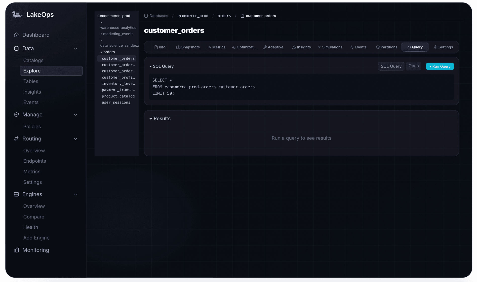
Every Iceberg query — Trino, Spark, DuckDB, Athena, Snowflake — follows the same four stages. Optimization is not a bag of unrelated tips. Each technique reduces work at a specific stage so the engine touches the minimum data required to answer the query.
Stage 1: Metadata resolution
The engine asks the catalog — Glue, REST, Polaris, Nessie — for the current metadata pointer. One RPC. Fast, but it pins the snapshot the query will read. Catalog latency is in every query's critical path.
Stage 2: Scan planning
The engine walks the snapshot's manifest list, then each manifest, collecting per-file statistics: partition values, row counts, column min/max, null counts. Predicates prune files that cannot contain matching rows.
This is where healthy and degraded tables diverge. Two hundred well-sized files: planning in milliseconds. Fifty thousand small files: the planner reads and evaluates thousands of manifest entries — 10–30 seconds, often longer than the scan itself.
Stage 3: File I/O
Surviving files are read from object storage. Parquet column projection means only referenced columns come off S3. Row-group min/max statistics prune inside files. File size is the tradeoff: too small and per-file HTTP/TLS/GET overhead dominates; too large and a selective query still reads more than it needs.
Stage 4: Processing
Filters, joins, aggregations. This stage is what engine vendors optimize hardest. By the time you are here, earlier stages have already decided how much unnecessary data the engine must chew through.
The optimization principle
Iceberg performance means less work at each stage. Fewer files → faster planning. Sort aligned to predicates → more pruning. Compact manifests → less metadata I/O. The right engine → the right execution profile. Every section below maps back to that principle.
The five degradation surfaces
Production tables degrade along five surfaces. Each maps to a stage in the pipeline. They compound: more files inflate manifests; slower planning delays maintenance; delayed maintenance creates more files.
1. File fragmentation
Every commit adds files. Streaming at 5-minute intervals produces ~8,600 files per table per month, typically 5–20 MB each. Engines perform best in the 256–512 MB range — large enough to amortize open cost, small enough that selective queries stay cheap.
At 50,000 files the engine opens 50,000 connections and schedules 50,000 tasks. The same bytes in 500 files is two orders of magnitude less coordination. File count — not data volume — is the usual reason Iceberg queries go slow.
2. Sort order misalignment
Parquet stores column min/max in file metadata. When files are sorted on the columns queries filter, each file's range is narrow. country = 'DE' skips every file whose country range excludes DE. That is statistical pruning: 90%+ of files never opened on a selective query.
Unsorted files (or files sorted on the wrong columns) span the full domain. Nothing prunes. The engine reads everything. A well-sorted table is typically 8–12x faster on those queries — and the gap is invisible unless you inspect file-level stats.
Sort order is not a one-time DDL choice. Dashboards ship, reports retire, agents start filtering on different columns. Last year's sort key silently stops matching this year's predicates.
3. Metadata bloat
Commits grow the manifest tree. Manifests fragment: many small files pointing at a mix of live and obsolete data files. At petabyte scale, 200,000 data files can mean 2,000 manifests and hundreds of megabytes of planning I/O.
Manifest rewrite consolidates that tree and can cut planning time 50–80%. It has to run after compaction (so it does not index files about to disappear) and before statistics refresh (so stats describe the new layout).
4. Delete-file debt
UPDATE, DELETE, and MERGE INTO do not rewrite data files. They write positional delete markers. Every reader reconciles markers against data at read time.
A CDC table at 50,000 updates/hour accumulates thousands of markers per day. Latency rises 2–5x while row count and table size look stable. Basic monitoring misses it. Iceberg V3 replaces position deletes with deletion vectors — binary bitmaps stored in Puffin files that flatten per-query reconciliation cost — but the underlying debt still accumulates and still requires periodic compaction to resolve. The fix is a targeted rewrite of the partitions that hold the debt — a compaction decision, not a monitoring dashboard.
5. Engine selection mismatch
The same SQL can differ 10–100x by engine. A 5-row lookup on Spark pays cluster startup; on DuckDB it returns in hundreds of milliseconds. A wide aggregation that crashes DuckDB finishes on Spark.
Most production lakehouses run several engines. If every query goes to whichever JDBC string the BI tool was given, you systematically pick the wrong latency and the wrong bill.
Compound degradation
These surfaces feed each other. More files → larger manifests → slower planning → slower maintenance → more files. Once the loop starts, it accelerates. Isolated fixes (nightly bin-pack, a static sort key, a weekly expire job) treat one surface and leave the loop intact. The architecture decisions that impact performance are rarely visible in a single query profile — they live in the coupling between surfaces.
Add an intelligent control plane
The highest-leverage change is architectural: a control plane that optimizes all five surfaces together, in dependency order, per table.
In Kubernetes the control plane observes cluster state and reconciles toward desired state without replacing the nodes. Applied to Iceberg: observe table health across catalogs and engines, decide what each table needs, execute the right sequence, and learn from outcomes. It does not replace your catalog, engines, or storage.
LakeOps is that layer for Iceberg lakehouses. It attaches to catalogs and engines you already run. No data movement, no pipeline rewrite. The point of introducing it here — before the per-surface deep dives — is that the surfaces are coupled. Bigger unsorted files do not prune. Sorted data behind bloated manifests still plans slowly. Manifests rewritten before delete resolution go stale immediately. Routing to DuckDB does not help if the table is a 50,000-file scan.
The intelligence is in the data, not the automation. The control plane collects cross-engine query telemetry — every predicate column, join key, and access frequency — and uses it to drive physical optimization decisions: which columns to sort on, which partitions to rewrite, which file sizes to target, which engine to route each query to. That is what makes it a control plane rather than a better cron. The rest of this guide is what each surface requires — and how those decisions actually work.


Surface 1: File layout
File layout is the foundation. Planning cost, prune effectiveness, and delete resolution all assume files are the right size and in the right places.
Bin-pack vs sort
Bin-pack merges small files toward a target size without changing row order. File count drops. Planning and open cost drop. Pruning does not improve — values inside each file are still scattered.
Sort compaction rewrites files in column order. Sort by event_date and a day filter reads one or two files instead of the table. For tables where queries spread across 3–4 filter columns unpredictably, Z-order (bit-interleaved multi-dimensional clustering) is the better choice — more expensive to write, but it prunes across all clustered columns simultaneously. Linear sort or Z-order, the correct strategy is usually sort-based, not bin-pack: 5–10x better on selective SQL. The hard part is knowing which columns.
Sizing
- 256 MB — default for mixed selective and wide scans.
- 512 MB — fewer files for heavy aggregations and full scans.
- 128 MB — when predicates are extremely selective and a 512 MB hit wastes I/O.
A static lake-wide target is wrong. Streaming bronze and daily gold do not share a file-size optimum. LakeOps compaction sets targets from query shape, access frequency, and engine mix per table.
What matters is cadence, not a nightly Spark job. If compaction is expensive, teams run it in an overnight window and live with 23 hours of drift. If it is cheap and fast enough to run when health signals fire, files never pile up. That is an execution-intelligence problem — covered when the control plane loop is spelled out below — not a target-file-size-bytes setting.
Surface 2: Sort order
For selective queries, sort order is the highest-leverage knob. Right columns make pruning surgical. Wrong columns make it theater.
Why manual sort keys fail
The right keys are the columns that actually appear in WHERE, JOIN, and GROUP BY — across every engine, not the one you happen to profile this week.
Trino filters customer_id. Spark joins event_date. A 50-column table has a huge sort space. A bad key wastes rewrite compute and can worsen pruning for half the workload. At a handful of tables you can guess. At hundreds, you cannot — and you will not notice until one dashboard is slow.
How the control plane chooses
The control plane aggregates predicate and join columns from Trino, Spark, Snowflake, Athena, DuckDB — every WHERE, JOIN, and GROUP BY across every engine reading the table. It scores candidate sort keys by projected scan reduction for the real query mix, not a single engine's EXPLAIN.
Concrete example: telemetry shows 70% of queries on a table filter event_date and 25% filter customer_id. The control plane sorts on event_date, customer_id. After compaction, each file holds a narrow date range. A date-filtered query that previously opened 500 files now opens 3 — a 99% reduction in file I/O, which directly cuts S3 GET costs, planning time, and CPU. When a new dashboard ships that filters region instead, the score updates and the next compaction cycle adjusts the sort key — no human editing YAML.
Simulate before rewrite
A production rewrite is expensive. The control plane replays real queries against candidate layouts on Iceberg branches and measures scan reduction first. Bad sorts die in simulation.

Partitioning is the other half of layout
Hidden partitioning lets you evolve specs without rewriting history. Start coarse (day, region). Over-partitioning creates thousands of tiny partitions, each with a handful of small files — fragmentation nested inside the partition scheme.
Surface 3: Metadata health
Metadata is the index that makes pruning possible. When the index is fragmented, every query pays — even if data files are perfect.
Manifests after files, not before
Rewrite manifests so they describe the current file set: fewer, larger manifests clustered with the compacted layout. Do it after compaction or you index files that are about to vanish.
Snapshots before orphans
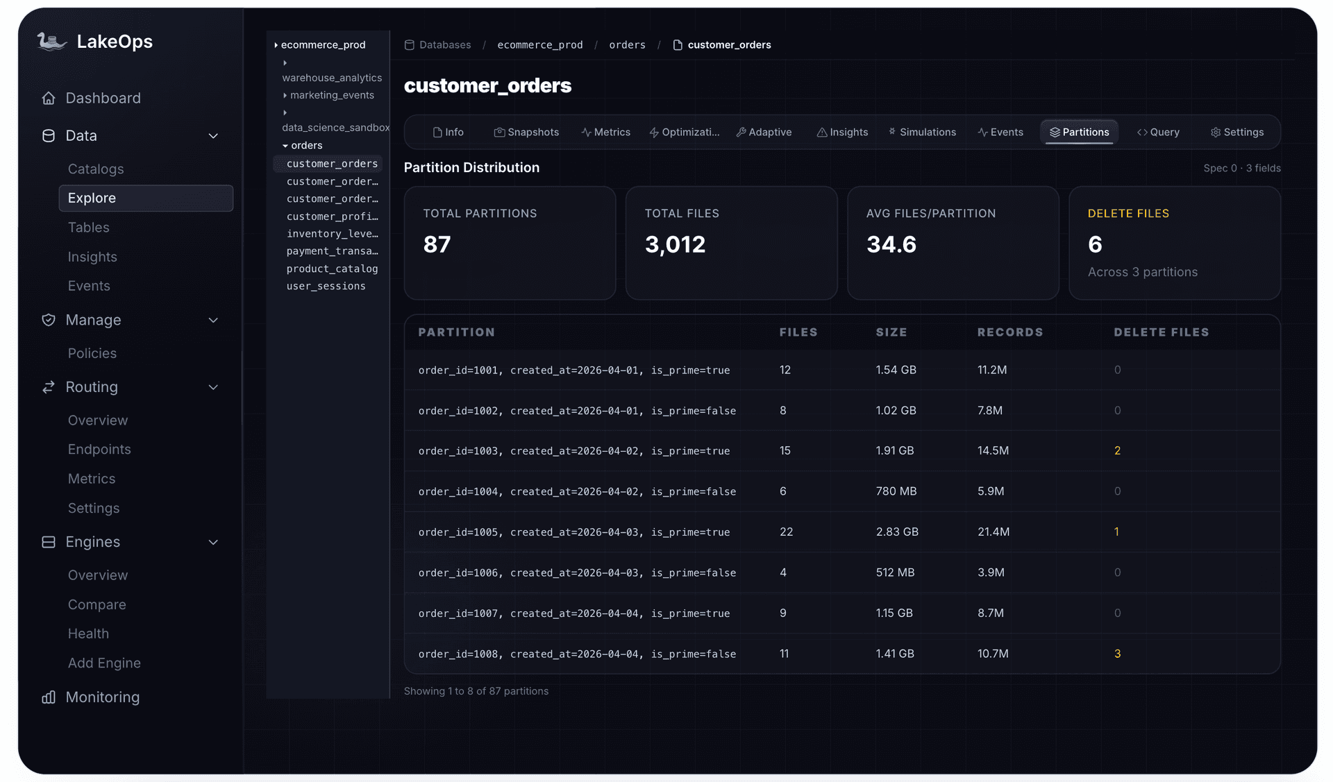
Each write is a snapshot. A daily 50 GB refresh is 365 snapshots a year and ~18 TB of logically replaced files until expiry. Expire first (dereference), then orphan cleanup (delete unreferenced objects). Reverse that order and you miss what you just freed.
Statistics last
Puffin NDV sketches and histograms improve join order and cardinality estimates in Trino and Spark. They must be recomputed after the files they describe have changed.
Managed maintenance is this sequence as one decision per table — expire → orphans → compact/sort → manifests → stats — only on partitions that need it.
Surface 4: Delete-file resolution
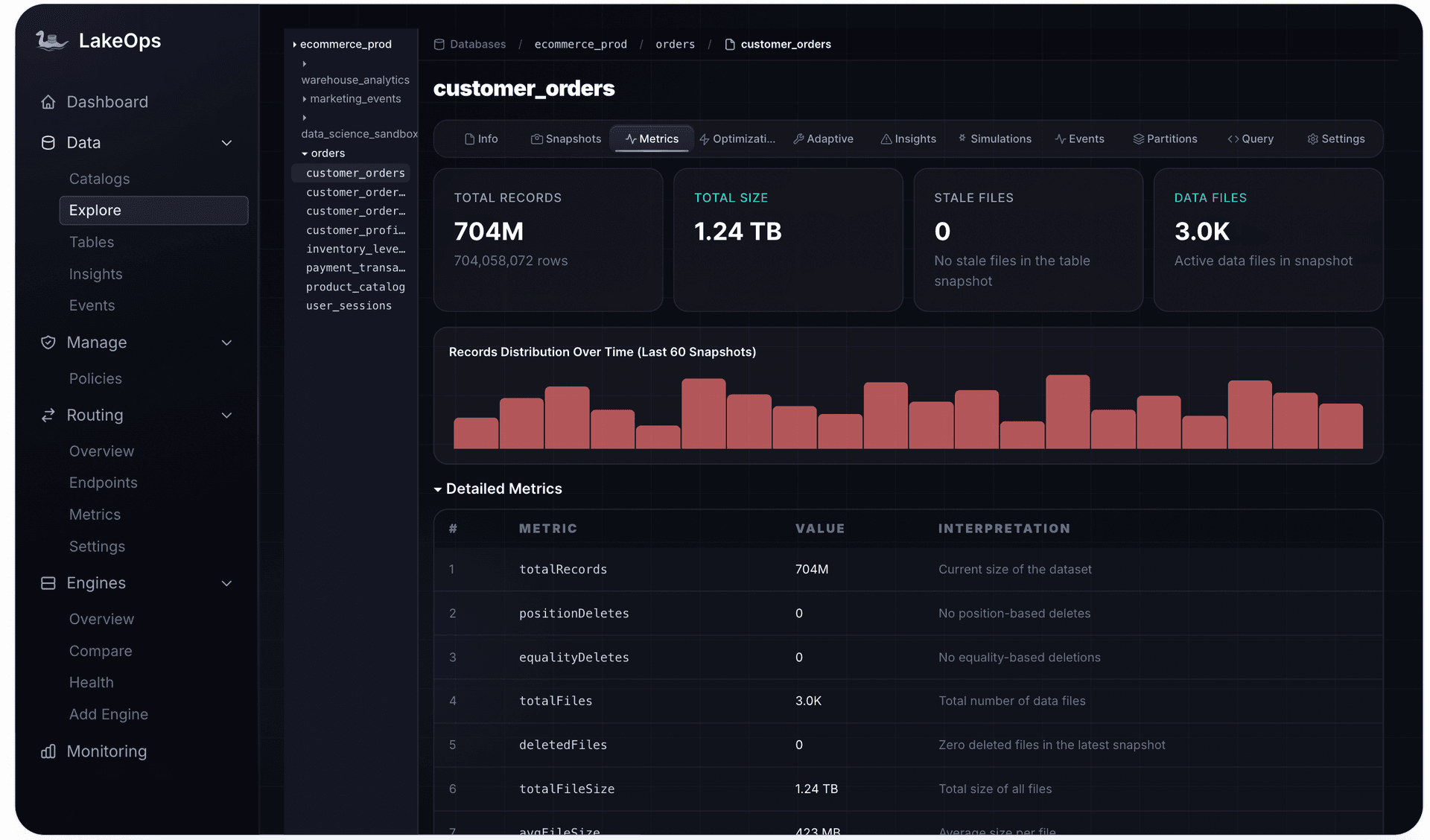
Delete files are the quiet tax. Row counts look right. Size looks stable. Every scan still merges markers.
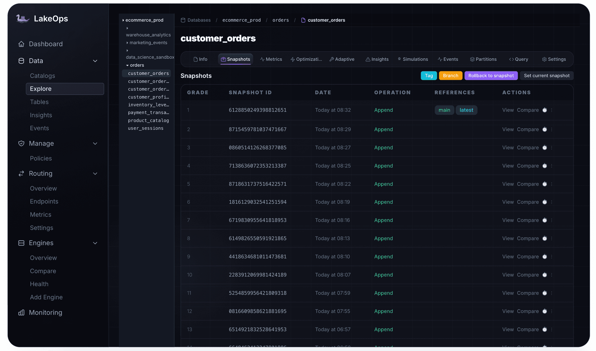
Iceberg keeps data files immutable. Mutations add position deletes. Low counts are cheap. Thousands per partition — normal for CDC — make reconciliation the dominant cost.
Resolution is physical rewrite of those partitions, not a full-table compact. The control plane ranks partitions by delete-to-data ratio and spends rewrite budget where read amplification actually is.
Surface 5: Engine routing
Layout decides how much data a query could skip. The engine decides how that remaining work is priced and scheduled.
Typical shapes: point lookup → DuckDB; dashboard SQL → Trino; wide batch → Spark; high-concurrency BI → Snowflake or a dedicated Trino pool. Without a routing layer, the user's client picks the engine — which is rarely the right one.
LakeOps query routing is one SQL endpoint. Dispatch uses query shape, table health, and cost/latency targets. Groups (analytics, ETL, BI, reports) stay stable while backends change.
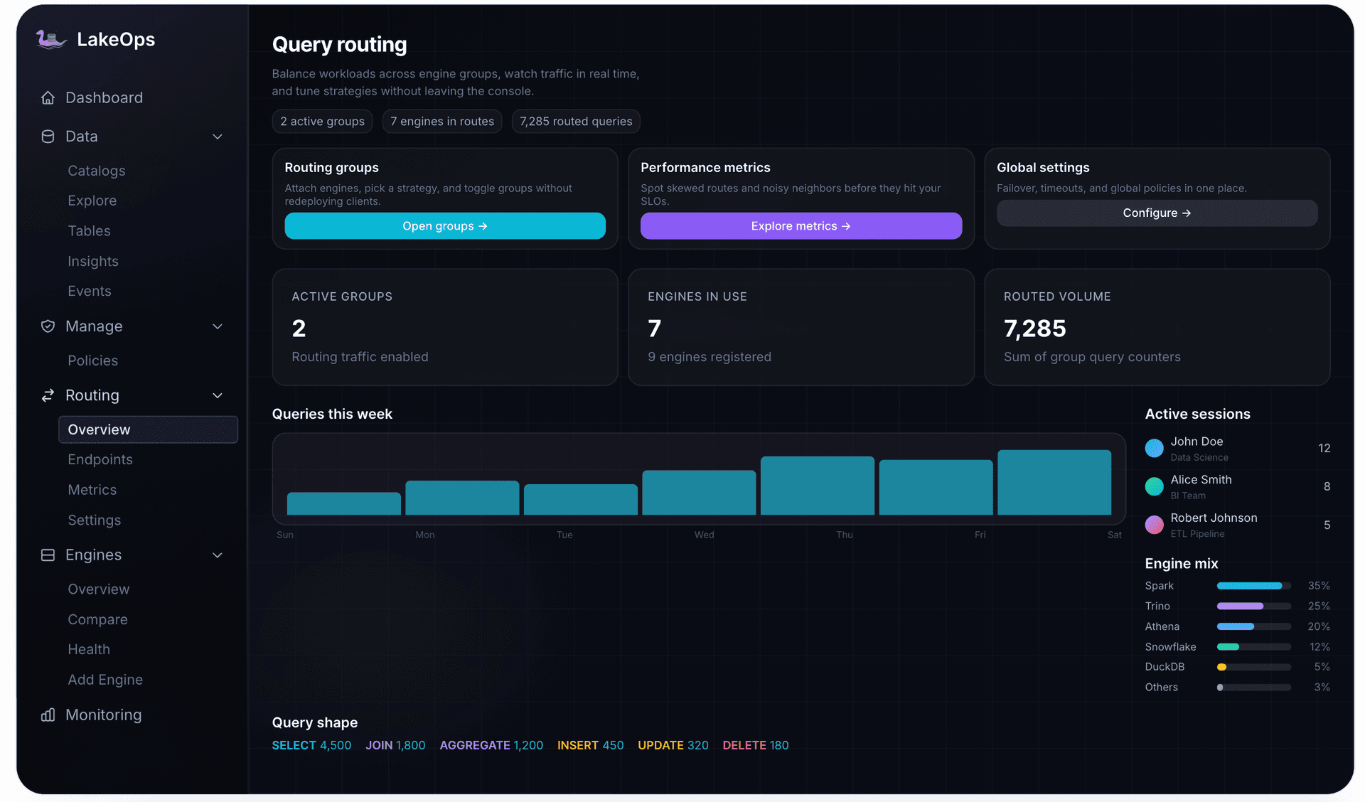

Maintenance and routing reinforce each other. Better layout makes more engines safe for a given query. More engines in play lowers cost. Cheaper queries run more often. More queries produce better sort telemetry.
Why scripts do not scale
You can compact, expire, and pick a sort key by hand on 5–10 tables. At production table counts the failure modes are structural.
Different tables need different work. Hourly CDC compact + delete resolve. Weekly gold expire-first. Monthly dimensions. One cron is either waste or neglect.
Operations have a required order. Expire → orphans → compact → manifests → stats. Independent jobs invert that and redo work.
Thresholds rot. “Compact above 1,000 files” was right for last quarter's cardinality. It is wrong after a partition evolution or a new stream. Nobody retunes until users complain.
No engine sees the full query mix. Trino's columns are not Spark's. A sort that helps one hurts the other unless telemetry is merged.
How the control plane actually runs
The LakeOps control plane is a closed loop: sense → assess → plan → execute → learn. Each phase exists because the failure modes above are coordination problems, not missing ALTER TABLE syntax.
Sense
Metadata only — file counts and sizes per partition, manifest depth, snapshot velocity, delete ratios, cross-engine predicates. No table data is read or moved.
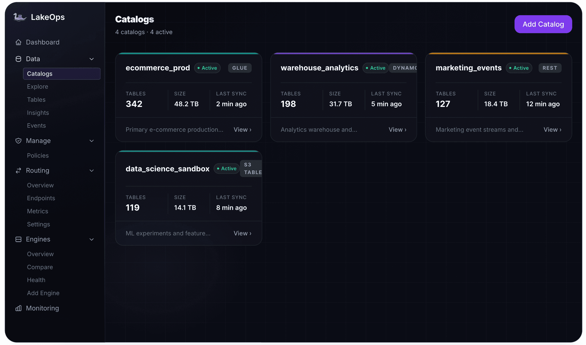
Passive, cheap, lake-wide. No single engine or catalog has this picture alone.
Assess
Telemetry becomes Healthy / Warning / Critical from file-size vs target, manifest compactness, delete ratios, sort-vs-predicate alignment, snapshot growth, and partition skew.

Thresholds are per table. A hundred commits an hour is not the same “healthy file count” as a daily batch. Observability is this classification with drill-down, not a generic metrics page.
Plan
Warning and Critical tables each get a tailored plan — not a generic schedule. A CDC table with 5,000 delete files gets rewrite priority. A streaming bronze table with 40,000 small files gets compaction first. A daily gold table with expired snapshots gets expiry before anything else. The order within each plan follows dependency:
Expire snapshots beyond retention — shrink the file set the later steps will touch. Remove orphans — unreferenced objects from failed writes and newly expired snapshots. Compact and sort — merge, apply deletes, sort on live query columns, only hot partitions. Rewrite manifests — index the new layout. Refresh statistics — pruning and CBO see current files.
Execute: intelligent, continuous optimization
Planning without execution is a ticket queue. The control plane runs the plan itself — and every execution decision is driven by the same telemetry that detected the problem.
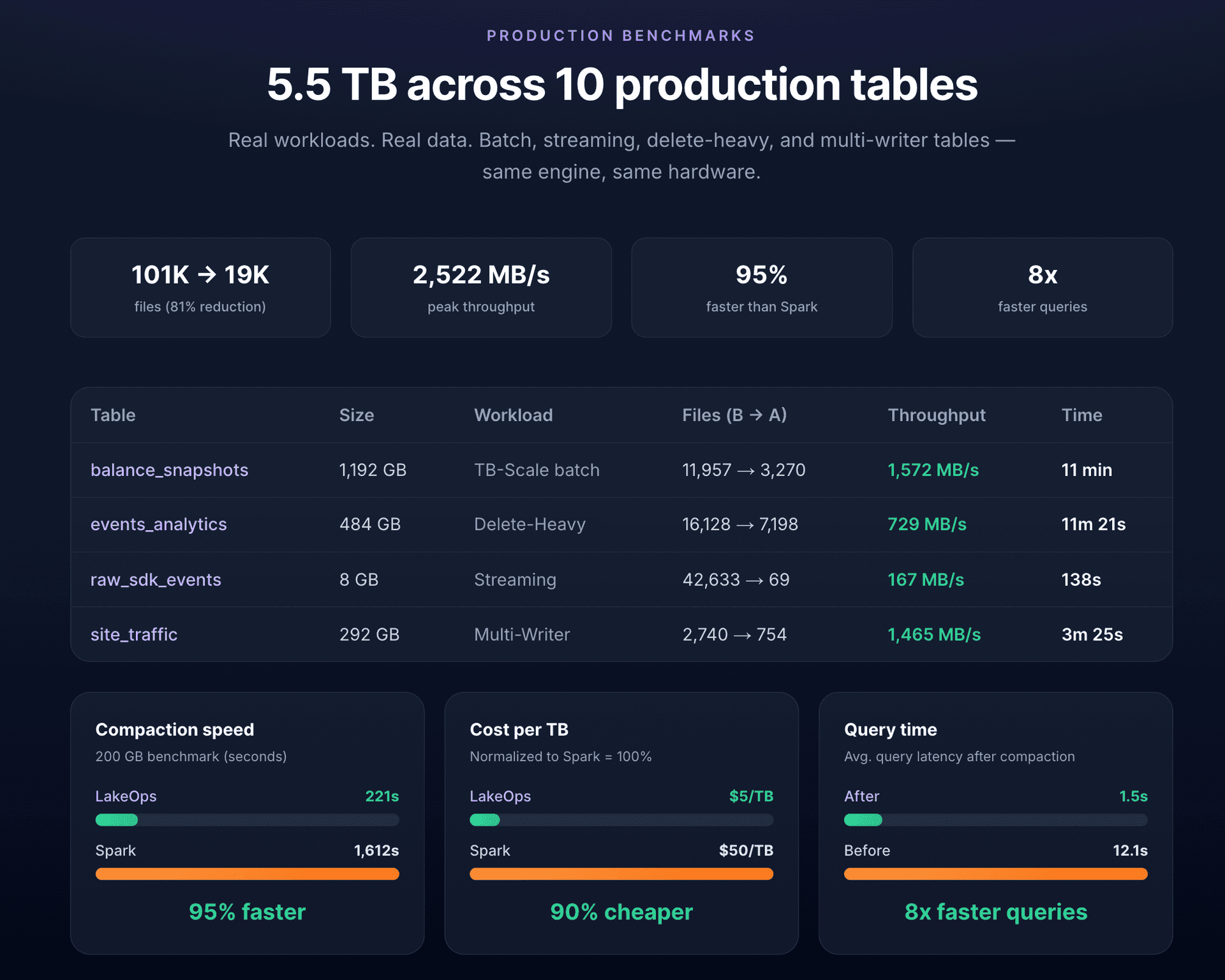
Compaction sorts on the columns production queries actually filter. Cross-engine telemetry feeds sort key selection. After a sort-compaction pass, file-level min/max ranges narrow from the full domain to tight bands. Statistical pruning goes from skipping 0% of files to skipping 90%+. That is an 8–12x drop in file I/O, S3 GET costs, and engine CPU — not from reading data faster, but from not reading it at all.
Delete resolution targets the partitions that cost the most. The control plane ranks partitions by delete-to-data ratio and rewrites the ones where read amplification is highest — not a full-table compact that wastes cycles on healthy partitions.
File sizing adapts to the table's query shape. Tables dominated by selective filters get 256 MB targets (fast prune, low waste). Tables serving wide aggregations get 512 MB (fewer files, fewer opens). The choice comes from access frequency and query type, not a static config.
Execution is conflict-aware. Partitions with active writers are skipped. Optimistic-concurrency retries happen automatically. Snapshots still held by readers are not expired. This is what makes continuous operation safe — and continuity is the point. If a cycle finishes before the next ingest wave, the five surfaces never compound. LakeOps compaction is built for that loop: maintenance is background reconciliation, not a weekend Spark job.: maintenance is background reconciliation, not a weekend Spark job. Tables stay fast because work happens before users feel Stage 2 planning blow up, not after.
Learn
After each cycle the control plane measures outcomes against the signals that triggered work: did file count hit target? Did planning latency drop? Did scanned bytes decrease in post-compaction queries? A sort on event_date that cut Stage 2 from 12 seconds to 200ms keeps its key. A sort that did not improve pruning gets replaced next cycle. Strategies evolve with the workload — without a human editing YAML.

Governance: policies that keep the loop honest
A control plane without policy is a well-intentioned autopilot. Defaults, namespace overrides, and table exceptions are how you keep retention, cadence, and risk aligned with the business:
- Organization defaults — compaction targets, snapshot retention, orphan windows
- Namespace rules — production aggressive; staging relaxed
- Table exceptions — 365-day compliance retention; 15-minute hot-table cadence
New tables inherit the namespace. Nothing waits to be added to a DAG.

Every run is logged: trigger, duration, bytes, files — the same audit trail shown above.
Optimization checklist
Use this whether you run a control plane or still own the jobs. Order is impact, then dependency.
1. Compact to target size. Kill small-file planning tax first. 256–512 MB. Often 3–5x on fragmented tables.
2. Sort on production predicates. Cross-engine WHERE / JOIN / GROUP BY. Typical 8–12x on selective SQL.
3. Resolve delete debt. CDC and MERGE tables: rewrite partitions above ~5–10% delete-to-data files.
4. Expire snapshots, then orphans. 3–7 days is enough for most tables. Expire, then cleanup.
5. Rewrite manifests after compaction. Index the new file set, not the old one.
6. Refresh statistics last. Puffin / engine ANALYZE on the compacted files.
7. Right-size partitions. Fewer than 5–10 files per partition usually means the spec is too fine. Evolve the partition spec.
8. Route by query shape. Lookup → DuckDB; dashboards → Trino; wide scans → Spark; concurrency → the engine that autoscale-fits.
9. Watch health continuously. Files/partition, avg size, deletes, manifests, snapshots, planning latency. Degradation is silent.
10. Automate the sequence. Manual: expire → cleanup → compact → manifests → stats. Better: let the control plane sequence it.
What the loop produces
When the five surfaces move together:
- Layout: 50,000 files → ~500. Planning 15s → <200ms.
- Sort: 8–12x on selective queries; bin-pack alone does not do this.
- Metadata: 50–80% less planning I/O after rewrite; 30–60% storage back from expiry on daily gold.
- Deletes: 2–5x read-latency drop on CDC tables after partition-targeted rewrite.
- Routing: 40–60% less aggregate compute with 3+ engines.
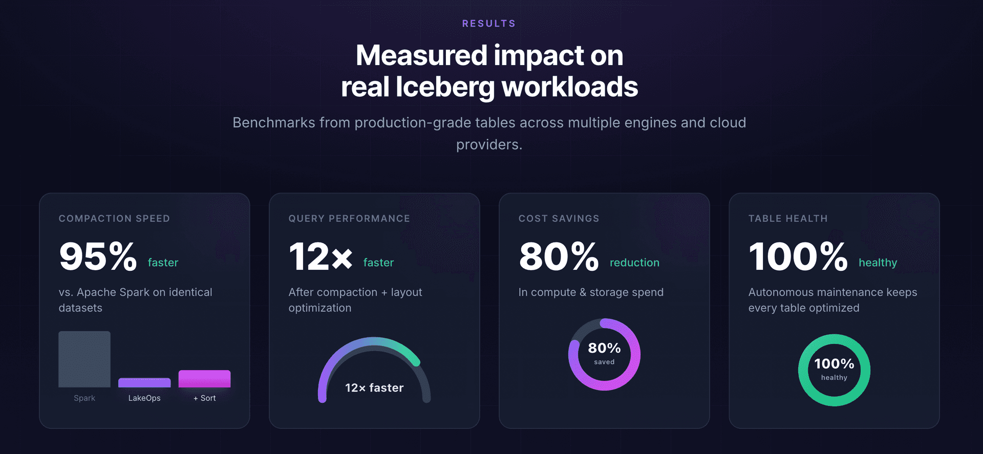
- Together: deployments at 500+ TB commonly report ~76% cost reduction and ~12x faster queries — because the loop compounds, not because one knob was maxed.
Implementing without boiling the lake
Each step has standalone value.
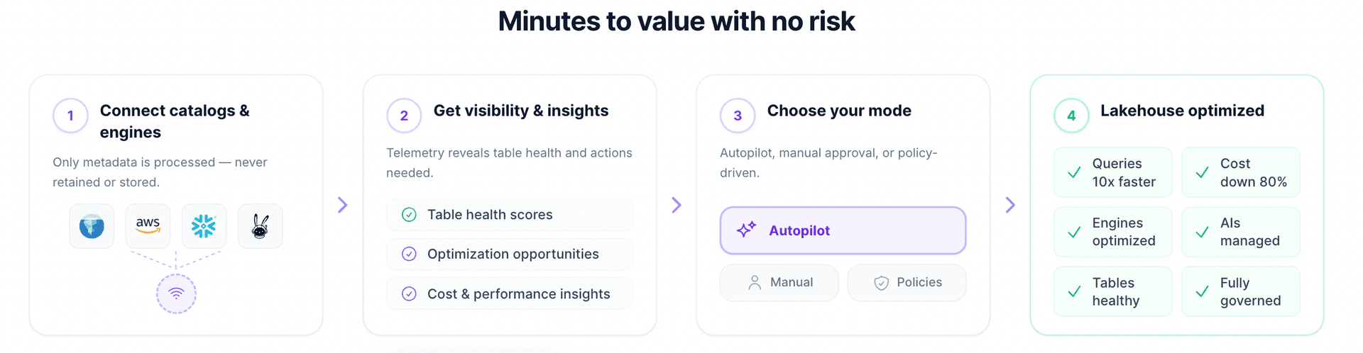
1. See state. Connect catalogs — minutes, no infra change. File counts, sizes, delete ratios, snapshot debt.
2. Compact the worst tables. Manual-approval first. Measure Stage 2 and Stage 3.
3. Turn on query-aware sort. After file counts stabilize. Simulate, then commit.
4. Autopilot the sequence. Autonomous mode once recommendations match what you would have approved.
5. Route. At 3+ engines, dispatch by shape.
Conclusion
Apache Iceberg performance is not a query hint and not a compaction cron. It is a property of the path from SQL to files: planning, layout, sort, metadata, delete markers, and engine choice. Those five surfaces degrade on a schedule you do not control, and they make each other worse.
You can tune each surface. The durable fix is to tune them together, in order, continuously. LakeOps is the control plane for that loop — sense structure, classify health, plan the sequence, execute only what changes query cost, learn from the next cycle.
Tables stay fast when something keeps the physical lake aligned with the queries that hit it. That is the job.
---
Further reading:
- Data Lakehouse with Apache Iceberg: A Guide — architecture layers and why tables degrade
- 9 Iceberg Compaction Tools Compared — engines and operators
- What Is a Data Lakehouse Control Plane? — the control-plane model
- Apache Iceberg Production Readiness Checklist — operational bar for production Iceberg