
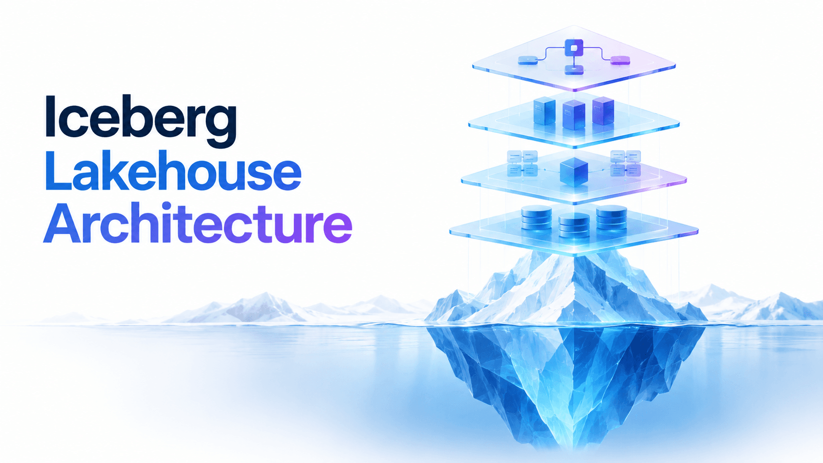
Every architecture diagram for a data lakehouse looks clean. Object storage at the bottom. Iceberg in the middle. Catalog above it. Engines on top. Draw the boxes, connect the arrows, done.
The problem is that this diagram describes a system at deployment time. It says nothing about the system at month six, when streaming jobs have created hundreds of thousands of small files, when query planning takes longer than the query, when storage costs have doubled from orphaned files that no component owns, and when three different engines are fighting over the same table's metadata.
The architecture is not wrong — it is incomplete. Apache Iceberg gives you transactions, time travel, and multi-engine access. What it deliberately does not give you is the operational intelligence to keep the system performing once real workloads hit it. That gap is architectural, not operational. And filling it requires a layer that most guides never mention. For the foundational concepts — the four layers, data flow, and why tables degrade — see our data lakehouse with Apache Iceberg guide.
This guide covers the full architecture — all five layers, from storage through the control plane. LakeOps is the control plane built for this — it connects to your existing catalogs and engines, adds the operational intelligence that Iceberg deliberately leaves out, and keeps every table healthy without moving data or changing pipelines. The guide explains what each layer does, what decisions to make at each one, how they interact, and where the architecture breaks down without the operational layer that ties everything together. It also covers the topics most guides skip: security across layers, migration paths from Hive and Delta Lake, data lifecycle management, and what Iceberg V3 changes at the format level.
Layer 1: Object storage
The lakehouse starts at the storage layer. All data — every row in every table — lives as files on cloud object storage: Amazon S3, Google Cloud Storage, or Azure Data Lake Storage. This is the foundational economic decision that makes the lakehouse viable.
Object storage provides eleven-nines durability at $20–25 per TB per month on standard tiers. A petabyte of analytical data costs roughly $20,000/month to persist on S3 Standard. The same data inside a traditional data warehouse with bundled compute runs $500,000+ annually. That cost difference is not an optimization — it is the entire economic rationale for the architecture.
A data lakehouse is not a data lake and not a data warehouse — it occupies a distinct architectural position. To understand where lakehouses fit versus lakes and warehouses, consider the economic and operational trade-offs at each layer. Storage is fully decoupled from compute. Shut down every query engine and the data remains exactly where it is. Spin up a new engine next month — it reads from the same bucket. Move clouds — the files copy byte-for-byte with no format conversion. This decoupling is what eliminates vendor lock-in at the deepest level of the stack.
Storage tiering and cost architecture
Not all object storage is priced equally, and the access-pattern economics matter more than most teams realize. On AWS S3 alone, you have several tiers with fundamentally different cost profiles:
- S3 Standard — $23/TB/month storage, $0.40 per 1,000 PUT requests, $0.0004 per 1,000 GET requests. Best for hot data accessed frequently by queries and maintenance.
- S3 Intelligent-Tiering — automatically moves objects between access tiers based on usage. No retrieval fees for frequent and infrequent access tiers. Adds a small monitoring fee per object. Ideal for tables with unpredictable access patterns.
- S3 Standard-IA (Infrequent Access) — $12.50/TB/month storage, but $10 per 1,000 GET requests. Looks cheap until you compact: rewriting 10,000 files means 10,000 GET requests at the IA price. A compaction pass that costs $0.04 on Standard costs $100 on IA.
- S3 Glacier Instant Retrieval — $4/TB/month, millisecond access, but $10 per 1,000 GET requests and $100 per 1,000 PUT requests. Suitable only for archival partitions that are rarely read and never rewritten.
The critical insight for Iceberg lakehouses: S3 API pricing amplifies the small-file problem. A table with 100,000 five-megabyte files costs 50× more in GET requests than the same data in 2,000 files at 256 MB — even when the storage cost is identical. Every query that plans against fragmented data pays the API tax. Every compaction run that reads and rewrites those files pays it twice. This is why small-file compaction is not just a performance optimization but a direct cost reduction.
For production lakehouses, the practical approach is tiered lifecycle rules: hot partitions (last 30–90 days) on S3 Standard, warm partitions on Intelligent-Tiering, and archival partitions on Glacier Instant Retrieval. But apply these rules at the partition level, not the bucket level — Iceberg's hidden partitioning makes this straightforward through S3 lifecycle policies scoped to partition prefixes.
The file format: Apache Parquet
Data lands as Apache Parquet files — a columnar format that stores values by column rather than by row. A query touching 5 columns from a 300-column table physically reads only those 5 columns. Parquet also embeds per-column min/max statistics in each row group footer, enabling query engines to skip entire row groups whose value ranges cannot satisfy the predicate.
Two properties of Parquet matter deeply for the layers above:
- Immutability. Parquet files are write-once. You never modify an existing file — you write new files and update the metadata layer to reflect the change. This is what makes ACID transactions possible on object storage without a database engine.
- Self-describing statistics. Each Parquet file carries its own metadata: schema, row count, column-level min/max values, null counts. These statistics are what the table format reads to decide which files to scan and which to skip — before opening any file for data.
The interplay between file size, sort order, and column statistics is where most lakehouse performance wins (and losses) originate. A well-organized collection of 256 MB Parquet files sorted by frequently-filtered columns enables engines to skip 90%+ of files on a typical query. The same data in 5 MB unsorted files forces a full scan. Same data, same engine, same query — 10× performance difference from layout alone.
Layer 2: The table format — Apache Iceberg
A directory of Parquet files on S3 is a data lake — readable, but not transactional. You cannot safely have two writers. You cannot roll back a failed write. You cannot evolve a schema without rewriting every file. You cannot ask "what did this table look like yesterday?"
The table format is the metadata layer that adds these guarantees. Apache Iceberg — the dominant open table format as of 2026, supported natively by every major query engine and cloud provider — provides ACID commits, schema evolution, time travel, hidden partitioning, and concurrent multi-writer safety through a metadata tree architecture that sits entirely on the same object storage as the data.
The metadata tree
Every Iceberg table is a tree of metadata files. Understanding this tree is the key to understanding both why Iceberg works and why it degrades.
1Catalog Pointer2 └── metadata.json ← current table state, schema, partition spec, sort order3 └── Snapshot ← immutable point-in-time version of the table4 └── Manifest List (.avro) ← indexes all active manifest files5 └── Manifest Files (.avro) ← per-file statistics6 └── Data Files (.parquet) ← actual rowsEvery write — INSERT, MERGE INTO, DELETE, UPDATE — produces a new snapshot. The snapshot points to a manifest list, which references manifest files, which track individual data files with per-file column statistics: path, partition values, row count, file size, column-level min/max bounds, null counts.
This structure is what gives Iceberg its power:
- Atomic commits. Each write creates new files and a new snapshot. The catalog atomically swaps the pointer from old snapshot to new. Readers always see consistent state. Failed writes leave no trace — the pointer was never advanced.
- Time travel. Old snapshots persist. Query any previous version by snapshot ID or timestamp. Roll back a bad write instantly by resetting the pointer.
- Schema evolution. Add, rename, drop, or reorder columns without rewriting data files. Each column has a unique ID — older files are read with the schema they were written under. For production patterns and pitfalls, see Iceberg schema evolution in production.
- Hidden partitioning. Partition transforms (day, month, hour, bucket, truncate) are metadata-level constructs. Queries never include partition columns in their SQL — the engine handles it automatically based on manifest statistics.
Iceberg V3: what changes architecturally
The Iceberg V3 format spec introduces several features that change how you architect and operate production tables:
Deletion vectors replace V2's position delete files. Instead of writing a separate Parquet file listing deleted row positions, V3 stores a compact bitmap (Roaring Bitmap) alongside each data file. The bitmap marks deleted rows inline — no separate file to open, no merge-on-read join. For CDC-heavy tables, this reduces the read amplification from updates by 2–4× compared to V2 position deletes. The operational implication: compaction still resolves deletion vectors (rewrites the file without the deleted rows), but readers pay far less penalty between compaction passes.
Puffin statistics files store advanced column-level statistics — NDV (number of distinct values), histograms, sketches — in a separate binary format alongside the metadata tree. Unlike Parquet footer stats (min/max only), Puffin stats enable true cost-based optimization: a query planner that knows a column has 50 million distinct values makes different join-ordering decisions than one that only knows the min/max range. Engines like Trino and Spark are progressively integrating Puffin-based planning, and keeping statistics current depends on maintenance operations that regenerate them after compaction.
Row lineage tracks the origin of each row across writes, enabling fine-grained audit trails and incremental processing patterns that previously required custom application logic. For compliance-heavy environments, row lineage means you can trace exactly which pipeline produced each row in the table.
The practical takeaway: V3 tables degrade differently than V2. Deletion vectors reduce read-side pain from unresolved deletes but still consume storage. Puffin statistics improve planning only when they're current — stale stats after a large write can mislead the optimizer. Both reinforce the need for continuous maintenance rather than reducing it.
The query path: how data skipping works
When a query hits an Iceberg table, the engine walks the tree top-down, pruning at each level:
Manifest list pruning. The manifest list contains partition summaries for each manifest. If a query filters on event_date = '2026-09-01' and a manifest's partition summary covers only June data, the engine skips the entire manifest without opening it.
Manifest file pruning. For each surviving manifest, the engine evaluates per-file column statistics. A data file whose customer_id range is 10000–19999 gets skipped when the query filters for customer_id = 42. This is where sort order matters: a sorted file has a tight min/max range; an unsorted file spans the entire column domain and can never be pruned.
Parquet row group pruning. Inside each surviving data file, Parquet organizes rows into row groups. Each row group carries its own column statistics. On a sorted file, row groups cover narrow value ranges and most get skipped. On an unsorted file, every row group spans the full domain.
This three-level pruning is the mechanism that makes lakehouse queries competitive with warehouse queries. But it works only when: (1) files are properly sized so the engine doesn't spend more time on metadata than on data, (2) files are sorted so column statistics are tight enough to enable skipping, and (3) manifests are consolidated so planning doesn't take longer than the query itself. Maintaining these conditions is the job of the layers above. For a deep dive on how pruning works at each level, see Apache Iceberg Query Planning Explained.
The critical implication: entropy
Every commit grows the tree. Every streaming micro-batch adds tiny files and a new snapshot. Every DELETE or UPDATE adds delete markers that readers must reconcile. Every schema change layers new metadata over old. Nothing is overwritten — immutability is the source of Iceberg's transactional safety and the source of every operational problem you will encounter in production.
From the first commit, an Iceberg table accumulates structural debt. The question is not whether the table degrades — it will — but whether something in the architecture actively counteracts it. This is where the control plane earns its place: LakeOps continuously monitors these structural signals — file count, size distribution, delete-file ratio, manifest depth — and runs the right maintenance operations before entropy compounds into a performance crisis.
Layer 3: The catalog
The catalog is the coordination service that answers two questions: where is the current metadata pointer for each table, and how do multiple engines safely coordinate writes?
Every engine — Spark, Trino, Flink, DuckDB, Snowflake — consults the catalog before each read (to locate current metadata) and during each write (to commit atomically via compare-and-swap). Without the catalog, concurrent writers could corrupt table state. With it, they race safely through optimistic concurrency control: one commits, the other retries against updated state.
The REST Catalog specification
The most consequential decision in Iceberg's ecosystem was the standardization of the REST Catalog specification — a standard HTTP API that every engine implements. Adding a new engine to your lakehouse is a configuration change (point it at the catalog URL), not an integration project.
Catalog options in 2026
The catalog landscape has matured significantly. Each option has distinct strengths, and the right choice depends on your cloud footprint, governance requirements, and team maturity. For a detailed evaluation of all seven major options, see the best catalog for Iceberg comparison:
- Apache Polaris — graduated as an ASF Top-Level Project in February 2026 (originally open-sourced by Snowflake as Polaris Catalog). The reference REST catalog implementation. Supports RBAC, credential vending, namespace-level access control. Production-grade and cloud-agnostic. The safest default choice for teams building a new multi-engine lakehouse.
- AWS Glue Data Catalog — the default for AWS-native stacks. Now supports the REST catalog API (not just the legacy Hive Metastore interface), which means non-AWS engines like Trino and Flink can connect through the standard REST protocol. Deeply integrated with IAM for access control. The pragmatic choice if your entire stack is on AWS and you want to minimize operational surface area.
- Amazon S3 Tables — Iceberg built directly into S3 as a storage-native feature. S3 Tables manages the catalog, stores data in an optimized format, and runs automatic compaction. The trade-off: you gain zero-ops table management but lose some control over compaction parameters, sort order, and cross-cloud portability.
- Project Nessie — Git-like branching and tagging for your data catalog. Create a branch, test a schema change or bulk load against real data, merge if it works, discard if it doesn't. Powerful for data engineering workflows that need staging environments. Built on the Iceberg REST spec.
- Apache Gravitino — multi-catalog federation under the Apache Software Foundation (originally from Datastrato). If you run Glue in us-east, Polaris in eu-west, and Nessie for staging, Gravitino provides a single unified namespace across all of them. Essential for multi-cloud and multi-region deployments.
- Lakekeeper — a Rust-native, cloud-native REST catalog built for performance and operational simplicity. Lightweight deployment, fast metadata operations, native support for credential vending and remote signing.
Credential vending and remote signing
One of the most important architectural shifts in the catalog layer is credential vending — the catalog issues short-lived, scoped storage credentials to engines at query time instead of engines holding long-lived S3 keys. When a Trino worker needs to read files from s3://warehouse/events/, it asks the catalog for temporary credentials scoped to exactly that prefix. The credentials expire in minutes.
This eliminates the need for broad IAM roles on compute clusters, reduces the blast radius of a compromised engine, and centralizes access control in the catalog where it belongs. Remote signing goes further: the engine sends unsigned S3 requests to the catalog, which signs them server-side — the engine never sees storage credentials at all.
Both features are part of the REST catalog spec and are supported by Polaris, Lakekeeper, and Gravitino. AWS Glue achieves similar scoping through IAM session policies. If you are building a new lakehouse in 2026, credential vending should be a non-negotiable requirement for your catalog choice.
Server-side scan planning
Traditionally, Iceberg scan planning happens client-side: the engine downloads manifest lists and manifest files, evaluates partition and column-level predicates, and builds the list of data files to read. For a table with 100,000 files, this means downloading and parsing hundreds of megabytes of Avro manifests before the first data byte is read.
Iceberg 1.11 introduced server-side scan planning through the REST catalog API. The engine sends the query's filter predicates to the catalog server, and the server returns only the list of matching data files — the engine never downloads the raw manifests. This shifts the planning cost from every client to a single server, dramatically reduces planning latency for large tables, and enables the catalog to cache planning results across queries.
Server-side planning is especially impactful in multi-engine environments. Instead of five engines each downloading and parsing the same manifests, one catalog server plans once and serves all five. The reduction in S3 GET requests alone can be significant at scale.
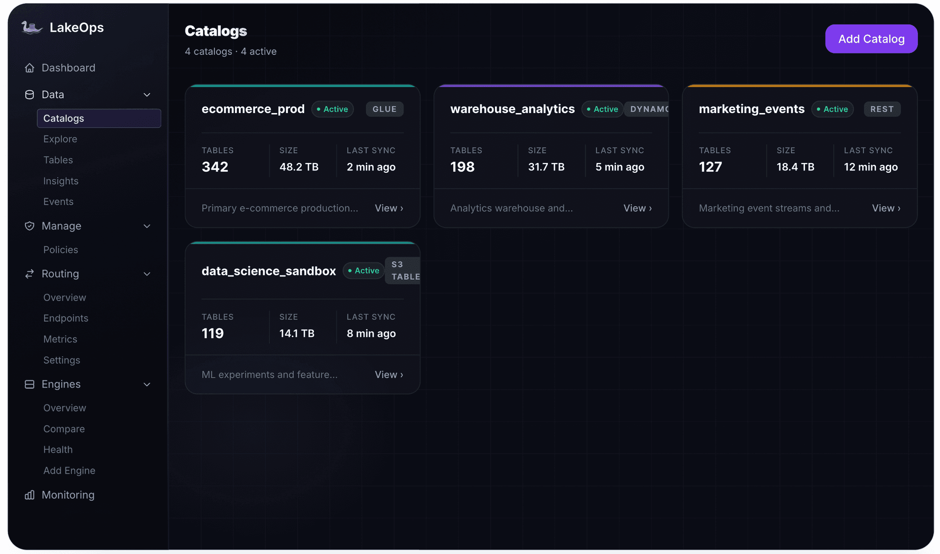
The practical recommendation for new deployments: use a REST-compatible catalog with credential vending support. It gives you engine portability, security, and planning efficiency from day one. If you are multi-cloud or multi-region, federate with Gravitino rather than running separate catalogs per environment. Whichever catalog you choose, LakeOps connects to it — Glue, Polaris, S3 Tables, Nessie, Gravitino, Lakekeeper — and gives you unified observability and maintenance across all of them through a single pane of glass.
Layer 4: Compute engines
The lakehouse separates compute from storage, enabling multiple specialized engines to operate on the same tables concurrently. This is the key architectural advantage over the data warehouse: instead of one vendor's engine for everything, you use the best tool for each workload shape.
- Apache Spark — batch ETL, ML training, complex multi-stage transformations. The workhorse for heavy writes and joins. Also the only engine that natively exposes Iceberg's maintenance procedures (
rewrite_data_files,expire_snapshots, etc.). - Trino — interactive SQL with sub-second response times. Excels at dashboard queries and ad-hoc exploration across large tables.
- Apache Flink — streaming ingestion with exactly-once semantics. Continuous CDC from operational databases into lakehouse tables. Checkpoint-aligned Iceberg commits.
- DuckDB — embedded analytics for notebooks, CI/CD pipelines, local development. Zero infrastructure overhead, runs in-process.
- Snowflake — managed engine with Iceberg Tables support (external tables backed by your S3 storage). High-concurrency BI workloads with zero cluster management.
- Amazon Athena — serverless ad-hoc queries. No infrastructure to manage, pay per query. Best for infrequent exploration and cost-sensitive workloads.
- StarRocks — real-time OLAP with materialized views over Iceberg tables. Sub-second aggregation queries at high concurrency.
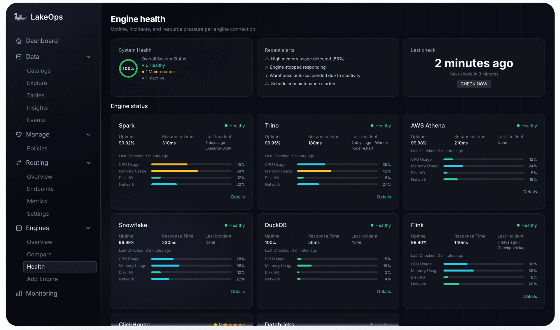
Each engine discovers tables through the same REST catalog and reads/writes through Iceberg's transactional protocol. They coexist safely on the same tables through snapshot isolation. A Flink job can stream writes while Trino serves dashboard queries and Spark runs an ETL pipeline — all hitting the same table, all seeing consistent state.
Practical engine selection criteria
Choosing engines is not about picking the best one — it is about matching engine characteristics to workload shapes. Here are the trade-offs that matter in production:
| Factor | Spark | Trino | Flink | DuckDB | Athena | Snowflake |
|---|---|---|---|---|---|---|
| Startup latency | 30–120s (cluster) | <1s (running) | N/A (always on) | <100ms | 2–5s | <1s |
| Best for | Heavy ETL, ML | Interactive SQL | Streaming | Local/embedded | Ad-hoc | High-concurrency BI |
| Cost model | Cluster hours | Cluster hours | Task slots | Free (in-process) | Per-query scan | Per-second compute |
| Write support | Full (MERGE, DELETE) | Limited | Append + CDC | Read-only* | Read-only | External tables |
| Maintenance | Native procedures | None | None | None | None | None |
| Scaling | Horizontal | Horizontal | Horizontal | Vertical (single node) | Automatic | Automatic |
The decision tree in practice: use Flink for streaming ingestion, Spark for heavy batch ETL and any write-intensive workloads, Trino for interactive queries from dashboards and analysts, DuckDB for lightweight local exploration and CI/CD data validation, and Athena or Snowflake for managed high-concurrency BI. Most production lakehouses run 2–3 engines concurrently — rarely just one, rarely more than four.
The multi-engine challenge
Multi-engine access is the architectural promise. Multi-engine coordination is the operational reality. Three practical problems emerge immediately:
Which engine should run which query? A point lookup on a well-sorted table finishes in 200 ms on DuckDB (no cluster needed) but takes 3 seconds on Spark (cluster startup). A 500 GB aggregation finishes in 45 seconds on Spark but OOMs on DuckDB. Without a routing layer, applications hardcode engine connections and every query goes to one engine regardless of fit.
Who owns table maintenance? Spark exposes the maintenance procedures, but running compaction on your query cluster steals resources from interactive users. Trino, DuckDB, and Athena don't expose maintenance procedures at all. If both Spark ETL and a separate Spark maintenance job try to compact the same table, they conflict.
Whose query patterns determine sort order? Trino dashboard queries filter on customer_id. Athena ad-hoc queries filter on event_date. Snowflake exploration filters on region. Each engine only sees its own query log. The optimal sort order depends on the combined query mix across all engines — which no single engine can observe.
These are not bugs — they are consequences of a deliberately decoupled architecture. Decoupling gives you freedom. It does not give you coordination. That requires a fifth layer — the control plane — which is exactly what LakeOps provides: cross-engine telemetry that informs sort-order selection, dedicated maintenance that doesn't steal query resources, and workload-aware routing that sends each query to the right engine automatically.

Why every lakehouse degrades
Before introducing the fifth layer, it helps to understand exactly why Iceberg tables degrade in production — and why no component in the four-layer architecture is designed to prevent it.
Degradation is not a failure mode. It is the natural consequence of an append-only transactional system under continuous workloads. Every Iceberg write creates new files and new metadata, and nothing in the stack removes the old ones. Four forces compound simultaneously:
File fragmentation. Streaming jobs committing every 30 seconds produce thousands of tiny files per day. Each file adds metadata overhead (manifest entries, Parquet footers, S3 API costs) and reduces query efficiency. A table with 100,000 files averaging 5 MB plans queries in 15–30 seconds. The same data in 2,000 files at 256 MB plans in under 1 second.
Delete file accumulation. Every UPDATE and DELETE in Iceberg V2/V3 writes markers that readers must reconcile against data files at read time. Merge-on-read is fast for the writer but expensive for every reader. A heavily-mutated CDC table accumulates thousands of delete markers — query latency increases 2–5× while the table's apparent size stays unchanged, making degradation invisible to basic monitoring.
Manifest proliferation. Each commit creates new manifest entries. A streaming table producing thousands of commits per day accumulates hundreds of megabytes of Avro metadata that query planners must parse before reading any data. Planning time alone can exceed 30 seconds on tables where the actual query would take 2.
Snapshot and orphan bloat. Without expiration, snapshots accumulate indefinitely — each one keeping its referenced files alive on storage, preventing garbage collection. Failed writes and aborted jobs leave orphan files on S3 that no snapshot references. These accumulate silently and show up only on the cloud bill.
These forces compound. More small files means more manifest entries. Larger manifests means slower planning. Slower planning means longer maintenance operations. Longer operations means less frequent runs. Less frequent runs means more degradation. The system has a natural tendency toward runaway entropy that accelerates once it begins.
And here is the architectural gap: no component in the four layers owns the fix. The storage layer just stores files. The table format provides maintenance procedures (rewrite_data_files, expire_snapshots, remove_orphan_files, rewrite_manifests) but does not schedule, coordinate, or trigger them. The catalog tracks metadata pointers but does not analyze them for health signals. The engines execute queries but do not maintain the tables they read. In a data warehouse, the vendor handles all of this invisibly. In an open lakehouse, the architecture deliberately leaves it to you.
Layer 5: The control plane
The first four layers give you a data lakehouse. The fifth layer is what makes it a production data lakehouse — one that stays fast, stays clean, and stays cheap without continuous manual intervention.
The concept comes from distributed systems. In a network, the control plane decides where traffic goes; the data plane moves packets. In Kubernetes, the control plane (API server, scheduler, controllers) observes cluster state and reconciles toward desired state. The data plane (kubelets, containers) does the work.
Applied to a lakehouse:
- Control plane — observes table health across the lake, decides what maintenance each table needs, executes it in the correct sequence, and verifies outcomes
- Data plane — the infrastructure: object storage, catalogs, engines
The control plane does not replace any existing layer. It adds the missing operational intelligence — the same way Kubernetes makes a container cluster self-healing without replacing Docker or the VMs underneath.
LakeOps is the control plane built for Apache Iceberg. It connects to your existing catalogs (AWS Glue, REST/Polaris, S3 Tables, Nessie, Gravitino) and engines (Trino, Spark, Snowflake, Athena, DuckDB, Flink) through standard APIs, without moving data or changing pipelines. It operates in a continuous closed loop — the Sense → Plan → Optimize → Learn cycle:
- 1.Sense — collects structural signals from every table (file count, file sizes, delete-file ratio, manifest depth, snapshot age, write velocity) and query telemetry from every connected engine (which columns appear in WHERE, JOIN, GROUP BY clauses).
- 2.Plan — scores each table as Healthy, Warning, or Critical. Determines which operations to run, in what order, with what parameters. Selects optimal compaction strategy and sort order from combined cross-engine telemetry.
- 3.Optimize — executes the sequenced maintenance pipeline on a purpose-built Rust engine powered by Apache DataFusion. Not on Spark — a dedicated engine with bounded memory, no JVM, no OOM. Correct sequencing is enforced: expire → orphans → compact → manifests.
- 4.Learn — measures outcomes and feeds results back. Sort orders adapt when query patterns shift. Compaction cadence tunes to write velocity. Adaptive scheduling adjusts to each table's actual behavior — streaming tables get compacted hourly, weekly batch tables once a week, idle tables are skipped entirely. Each cycle improves the next.
Setup takes about 10 minutes. Only metadata is processed — data never leaves your storage, is never copied, never retained. You choose how much control to keep: Autopilot (fully autonomous), Manual Approval (the system recommends, you approve), or Policy-driven (declarative rules that enforce themselves).

The rest of this guide walks through what the control plane actually does at each layer of the architecture — and how each capability maps to the operational problems described above.
Observability: seeing what is degrading
You cannot maintain what you cannot see. The first job of the control plane is to provide lake-wide visibility into every table's structural health — something Iceberg does not ship and no engine provides natively.
Iceberg exposes raw metadata through system tables (files, manifests, snapshots, history). You can write SQL to inspect any individual table. But raw metadata is not observability. Observability means: which of my 500 tables need attention right now, how urgently, and what specifically is wrong?
LakeOps scores every table continuously across six dimensions: file size distribution, small-file ratio, delete-file accumulation, manifest depth, snapshot age, and write velocity. Each table is classified as Healthy, Warning, or Critical. You see the entire lake at a glance — not one table at a time through ad-hoc SQL.

Proactive insights surface specific problems before users notice them: a partition exploding in file count, a manifest that has grown past planning thresholds, a table where delete files are adding 300+ ms of merge-on-read overhead per query. Each insight includes severity, the affected table and partition, and the recommended action.

Cross-engine telemetry aggregates query patterns from every connected engine into a single access profile per table. You see which columns are filtered, joined, and grouped — from Trino, Spark, Snowflake, and Athena simultaneously. This unified view is impossible to build from any single engine's query log.
Autonomous table maintenance
Iceberg ships four maintenance procedures. Running them correctly requires understanding their dependencies, sequencing them in the right order, and adapting cadence to each table's write velocity.
The correct sequence:
- 1.Expire snapshots — remove old snapshots and release the files they exclusively reference. Always first: if you compact before expiring, you rewrite files that expiration would have removed.
- 2.Remove orphan files — clean up files on S3 that no snapshot references (from failed writes, aborted jobs). Use a 72-hour grace period minimum to avoid deleting files from in-progress writes.
- 3.Compact data files — merge small files into optimally-sized ones, sort by query-relevant columns, resolve accumulated delete files. The most compute-intensive operation.
- 4.Rewrite manifests — consolidate fragmented manifests into fewer, larger ones aligned with partition boundaries. Metadata-only, cheap, outsized impact on planning time.
Each step's output is the next step's clean input. Expire first so compaction doesn't rewrite dead data. Compact before rewriting manifests so the manifest layout reflects the current file layout.
On the manual path, you build this as an Airflow DAG per table — four tasks, dependency-ordered, with error handling, retry logic, and Spark cluster management at every step. At 10 tables, it is manageable. At 200, the DAGs themselves become a maintenance burden — each one a production system that needs monitoring, alerting, and on-call coverage.
LakeOps runs this exact four-step pipeline automatically for every connected table. Operations fire based on health-driven triggers, not fixed cron schedules. A streaming table committing every 30 seconds gets compacted multiple times per hour. A weekly batch table gets compacted once. A table nobody writes to gets skipped entirely — zero wasted compute. The most degraded tables always run first.

Every operation is logged with full context: what ran, when, duration, files before and after, bytes reclaimed, and the health signal that triggered it. The audit trail is continuous and structured — essential for compliance environments that require proof of data lifecycle management.

Query-driven compaction
Standard compaction merges small files into bigger ones — bin-pack. That helps with file count but does nothing for data skipping. Query-driven compaction goes further: it learns which columns your queries actually filter, join, and group on, then physically re-sorts data files to match.
The difference is concrete. On a large table, bin-pack reduces file count — faster planning, fewer S3 requests. But a query filtering on customer_id = 42 still opens every file because no file's min/max range is tight enough to prove it doesn't contain that value. Sort compaction on customer_id produces files where each one covers a narrow ID range — the same query now opens a handful of files instead of thousands.
The hard part is choosing the right sort columns. And not just once — every time query patterns change, the sort order needs to change with them. A sort order chosen in January may not match the queries hitting the table in September because new dashboards, new teams, and AI agents all change access patterns.
LakeOps collects column-level access frequency from every connected engine — WHERE, JOIN, and GROUP BY predicates from Trino, Spark, Snowflake, Athena, DuckDB, and Flink simultaneously. It ranks columns by file-pruning impact and applies the optimal sort order during compaction. When patterns shift — a new BI dashboard starts filtering on region instead of customer_id — the sort order adapts on the next compaction pass.
Layout simulations
Sorting a terabyte table is expensive. If you pick the wrong columns, you pay the compute cost for zero benefit. LakeOps runs layout simulations on Iceberg branches — testing sort orders against real production queries without touching production data. Compare scan reduction, file count, and estimated query speedup side by side. Apply the winner. Production tables stay untouched until you are confident.

The Rust compaction engine
Compaction is a narrow, I/O-bound read-merge-write operation. Running it on Spark — a general-purpose distributed JVM engine — means paying for cluster startup, garbage collection pauses, executor overhead, and the ever-present risk of OOM on large sort operations.
LakeOps replaces Spark with a purpose-built Rust engine powered by Apache DataFusion: zero-copy Arrow columnar pipeline, bounded memory with disk spill, lock-free parallelism. No JVM, no GC, no cluster to provision. The engine learns from each run — consecutive passes on the same table improve throughput without configuration changes.
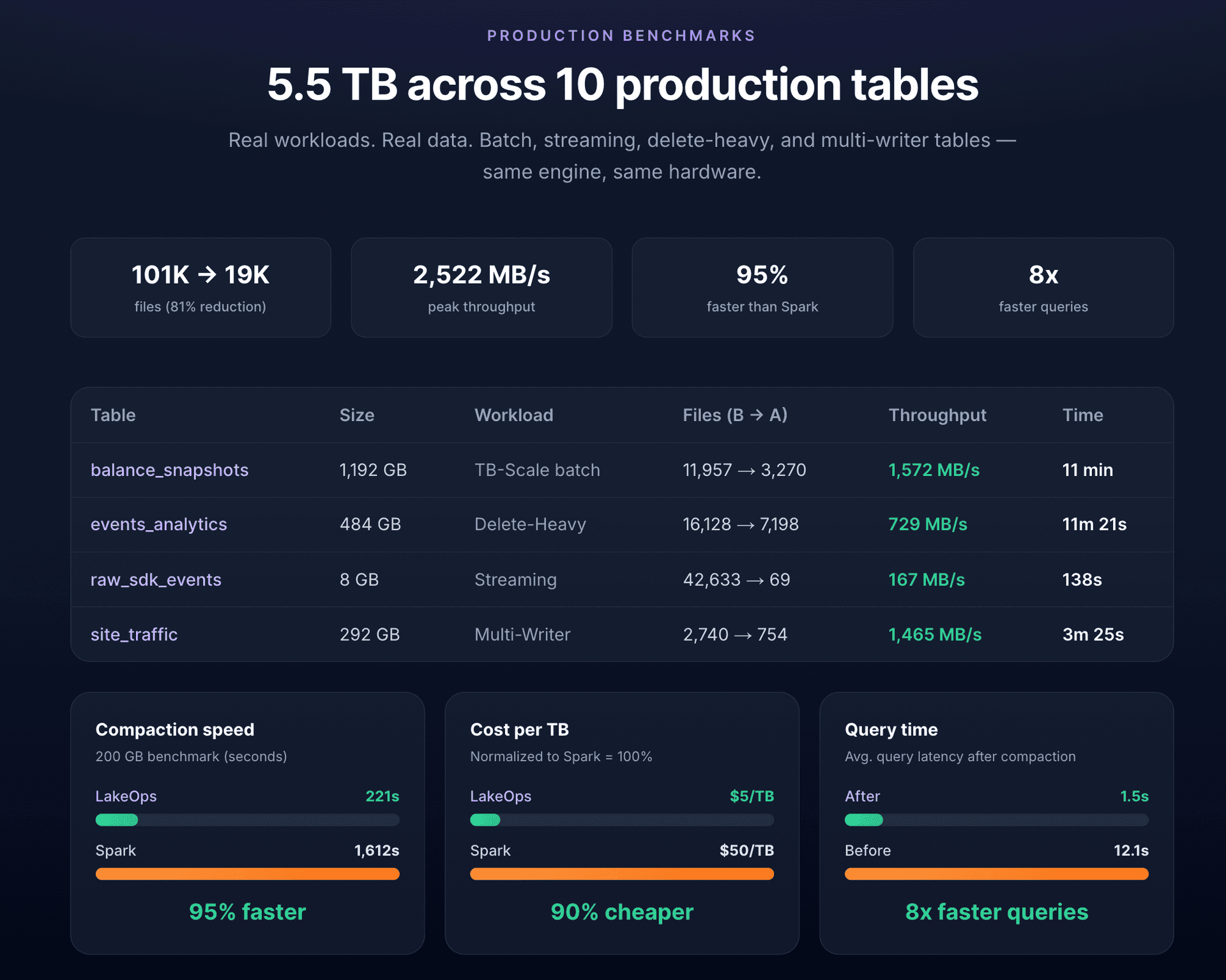
Production benchmarks on the same 200 GB / 600M-row table, same hardware: S3 Tables compaction took 6,300 seconds (~32 MB/s), Spark took 1,612 seconds (~350 MB/s), LakeOps finished in 221 seconds (2,522 MB/s). That is 95% faster and roughly 90% cheaper per TB ($5/TB versus $50/TB). Full benchmarks on the LakeOps compaction page.
Security architecture across layers
Security in a lakehouse is not a single feature — it is an emergent property of how all five layers enforce access control together. Each layer has its own security surface, and gaps between layers are where breaches happen.
Storage-layer security (IAM)
At the bottom, S3 bucket policies and IAM roles control who can read and write raw files. This is the coarsest level of control — you can restrict access to a bucket or prefix, but you cannot restrict access to specific rows or columns within a Parquet file. Storage-layer security is necessary but not sufficient. It is the last line of defense, not the first.
Catalog-layer security (RBAC and credential vending)
The catalog is where fine-grained access control lives. REST catalogs like Polaris and Gravitino support namespace-level and table-level RBAC: define which roles can SELECT, INSERT, or ALTER which tables. Combined with credential vending (discussed above), this means engines receive only the storage credentials they need for the specific tables the user is authorized to access.
For Iceberg lakehouses in 2026, the best practice is: define all access policies in the catalog, use credential vending to enforce them at the storage layer, and treat engine-level auth as a complementary (not primary) control. This is the "catalog as governance anchor" pattern.
Engine-layer security
Each engine has its own authentication and authorization mechanism — Trino has access control plugins, Spark has table ACLs, Snowflake has its own RBAC. In a multi-engine environment, maintaining consistent policies across engines is the practical challenge. A user blocked from a table in Trino should also be blocked in Spark and Athena.
The architectural answer is to push authorization down to the catalog layer (via credential vending) so that engine-level controls become defense-in-depth rather than the primary enforcement point. This avoids the "policy sprawl" problem where each engine has its own inconsistent set of access rules.
Control-plane security
The control plane itself needs strict access control. LakeOps operates on metadata only — it never reads, copies, or stores your actual data. SOC 2 compliance, SSO integration, and RBAC for platform operations (who can approve maintenance, who can change policies, who can view table health) ensure that the operational layer does not become a security gap. For organizations evaluating managed Iceberg solutions, the security posture of the control plane is a critical selection criterion.
Governance and policies
At 10 tables, you configure maintenance per table. At 500, you need policies. Declarative policies define maintenance rules at the catalog, namespace, or individual table level — everything cascades with inheritance.
A policy might say: "All tables in the analytics namespace target 256 MB file size, retain snapshots for 7 days, run orphan cleanup weekly, and use sort compaction with query-aware column selection." Set it once — every current and future table in that namespace inherits it automatically. No per-table onboarding, no forgotten configuration, no drift.
Policies cover compaction targets, snapshot retention windows, orphan cleanup thresholds, manifest optimization frequency, sort strategies, and alerting rules. All policies are versioned, auditable, and reversible — roll back any change with full visibility into what was changed and when.

Policy enforcement is where the control plane and governance intersect. LakeOps enforces declared policies through the Sense → Plan → Optimize → Learn loop — if a table violates its policy (file sizes exceeding targets, snapshot count over the retention limit, orphan ratio climbing), the system detects the drift and corrects it automatically. This is declarative governance: you state the desired state, the system enforces it continuously.
Multi-engine query routing
Production lakehouses run multiple engines. Without routing, applications hardcode engine connections — every query goes to one engine regardless of cost or latency characteristics. The result is either overspending (sending a simple lookup to Spark) or poor performance (sending a large join to DuckDB).
LakeOps provides query routing through named, workload-scoped endpoints. Each endpoint gives applications a stable URL, a defined engine pool, query-type scope, and priority level. An analytics endpoint routes SELECT and AGGREGATE queries to Trino + DuckDB. An ETL endpoint routes INSERT and MERGE to Spark. A BI endpoint routes to Snowflake with Trino fallback. Applications connect to their endpoint — the routing layer dispatches to the optimal engine based on query shape, cost ceilings, latency targets, and current engine availability.

The routing layer and maintenance layer form a reinforcing loop. Compaction and sorting unlock cheaper engines for more query shapes — a well-sorted table can serve lookups from DuckDB that a fragmented table cannot. Routing telemetry feeds back into compaction decisions — knowing which queries hit which tables informs sort-order selection. Both systems improve simultaneously.
Data ingestion patterns
The lakehouse architecture supports three ingestion patterns, each with different implications for table health and maintenance requirements.
Batch ingestion
Spark, dbt, or Airflow jobs run on a schedule — hourly, daily — and write large batches of rows into Iceberg tables. Each batch produces a small number of well-sized files. Maintenance is straightforward: run compaction and manifest rewriting after each load completes. The table degrades slowly between batches and recovers with each maintenance pass.
Streaming ingestion
Flink or Kafka Connect jobs write continuously with sub-minute commit intervals. This is the primary source of the small-file problem — a Flink job committing every 30 seconds to 4 partitions produces over 11,000 new files per day. The table degrades continuously and requires compaction multiple times per hour on cold partitions (those not actively being written to).
The critical streaming complication is optimistic concurrency control (OCC). If compaction tries to rewrite files in a partition that a streaming writer just modified, the compaction commit fails. The solution is partition-aware compaction — never compact the partition being actively written to. On the manual path, this means adding a WHERE event_date < current_date() clause and hoping for the best. LakeOps monitors actual per-partition commit activity across all engines and automatically excludes active partitions — protecting against backfills, late arrivals, and multi-engine writes that date-based filters miss.
CDC ingestion
Change Data Capture from operational databases (Debezium, Flink CDC, Kafka Connect) writes row-level changes — inserts, updates, and deletes — into Iceberg tables. Updates and deletes produce merge-on-read delete files (position deletes in V2, deletion vectors in V3) that readers must reconcile at query time. CDC tables need aggressive compaction with delete resolution to prevent merge-on-read overhead from accumulating. LakeOps monitors the delete-to-data ratio per partition and triggers compaction when the overhead crosses thresholds — resolving position deletes, equality deletes, and V3 deletion vectors in the same compaction pass.
Data lifecycle management
A production lakehouse is not just about ingestion and querying — it is about managing data through its entire lifecycle: from arrival through active use, archival, and eventual deletion. Iceberg's snapshot-based architecture gives you the primitives. The control plane turns them into enforceable policy.
Retention and archival
Snapshot retention determines how long you can time-travel and how much storage overhead you carry. But data retention goes deeper: which partitions should be archived to cheaper storage tiers? Which tables should be dropped entirely after a regulatory holding period expires? Which datasets need to be retained indefinitely for audit purposes?
Declarative policies in LakeOps handle this at the namespace level. Set a retention window per table class — hot analytics tables retain 90 days of snapshots, compliance tables retain 7 years of tagged checkpoints, staging tables expire after 48 hours. Policies cascade through inheritance and enforce themselves through the maintenance loop.
GDPR and physical erasure
GDPR's right to erasure creates a specific challenge for immutable storage. Iceberg never overwrites files — a DELETE writes new metadata, but the old Parquet file with the deleted rows persists until snapshot expiration garbage-collects it. "Logical deletion" (marking rows as deleted) is immediate. Physical erasure (removing the actual bytes from storage) requires: (1) deleting the rows, (2) compacting the affected files to produce new files without the deleted rows, (3) expiring all snapshots that reference the old files, and (4) running orphan cleanup to remove the old Parquet files from S3.
This is a four-step, dependency-ordered process — exactly the sequenced maintenance pipeline the control plane executes. For GDPR compliance, the critical metric is the time between the delete request and physical erasure of the underlying bytes. With LakeOps, this is deterministic and auditable: the policy defines the retention window, the maintenance loop enforces the expiration sequence, and the audit trail proves when the bytes were physically removed.
Snapshot management and time travel
Iceberg's snapshot chain enables time travel and consistent reads — but it is also the primary source of storage bloat when unmanaged. Each snapshot keeps its referenced files alive. Without expiration, a streaming table producing 3+ snapshots per hour accumulates thousands per month.
Snapshot retention is workload-specific:
- Streaming tables — 3–7 days, retain last 25–50 snapshots. Short retention because new snapshots arrive frequently and old ones lose relevance fast.
- Batch tables — 7–30 days, retain last 5–10 snapshots. Longer retention for rollback safety and audit requirements.
- Compliance tables — Use Iceberg tags on specific checkpoints (end-of-quarter, audit milestones). Tagged snapshots survive expiration automatically, giving you permanent bookmarks without keeping the entire chain.
The safety rule: set older_than to at least 2× the duration of your longest-running query. A read that opened a snapshot can fail if that snapshot gets expired mid-scan. Set retain_last to at least 2 — never 1, which leaves zero rollback targets.
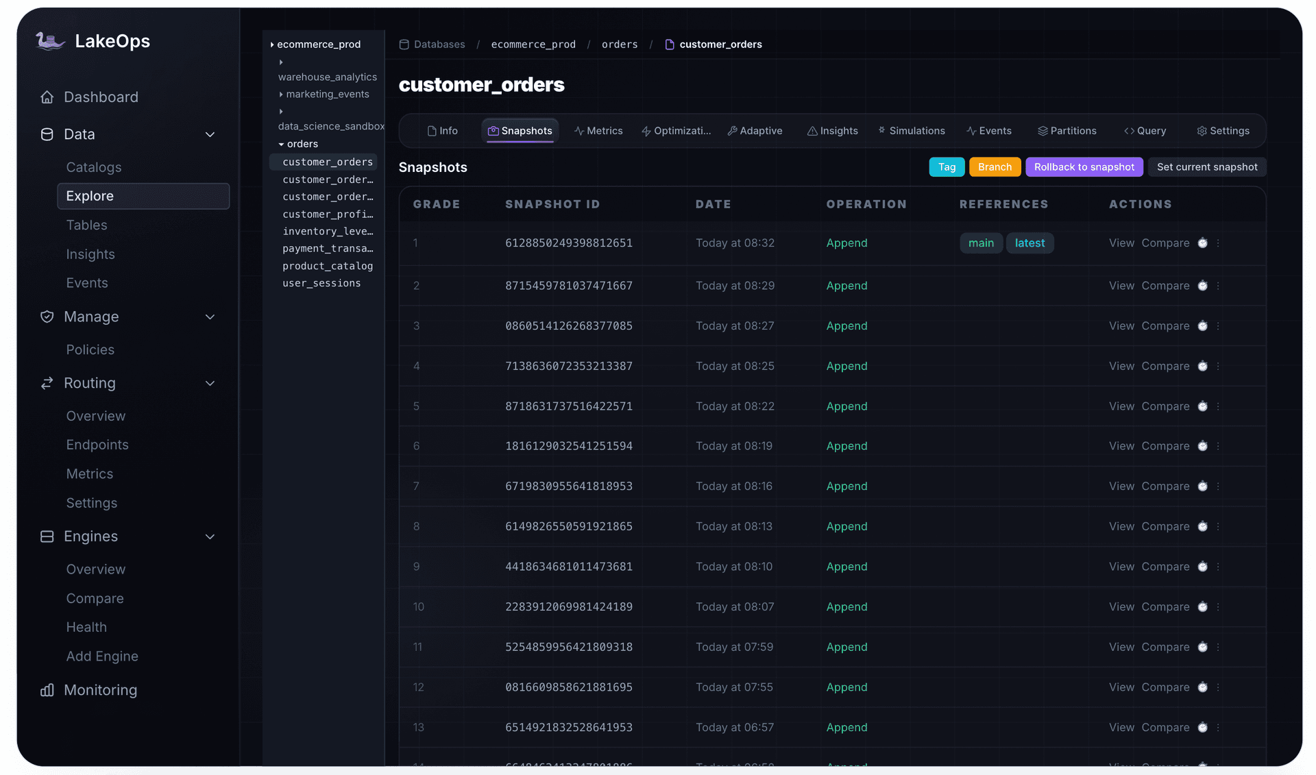
LakeOps handles snapshot expiration as part of the sequenced maintenance pipeline — always first, always before compaction — with retention windows configurable via declarative policies at the namespace level.
Migration paths: moving to Iceberg
Most organizations building an Iceberg lakehouse in 2026 are not starting from zero. They are migrating from Hive tables, Delta Lake, or a mix of both. Each migration path has distinct trade-offs.
From Hive tables to Iceberg
Hive tables are the most common starting point. The migration has two approaches:
In-place migration uses Iceberg's migrate procedure to convert Hive table metadata to Iceberg metadata without rewriting any data files. The existing Parquet files stay on S3; Iceberg creates new metadata (snapshots, manifests) that point to them. This is fast — minutes for even large tables — but you inherit whatever file layout Hive had: often unsorted, inconsistently sized, and partition-scheme-dependent.
Shadow migration creates a new Iceberg table alongside the Hive table, copies the data with the desired sort order and file sizes, and cuts over once validated. Slower, but you get a clean starting state with optimized layout.
The practical recommendation: use in-place migration to get tables into Iceberg quickly, then let the control plane compact and sort them into optimal layout over subsequent maintenance cycles. This gives you the fastest time-to-value without the risk of a big-bang rewrite.
From Delta Lake to Iceberg
Delta-to-Iceberg migration leverages the fact that both formats store data as Parquet files on object storage. The data doesn't need to move — only the metadata layer changes.
Delta Lake UniForm (Databricks) can generate Iceberg-compatible metadata alongside Delta metadata, enabling dual-format reads. This is useful as a transition mechanism but not a long-term architecture — you are still running Delta's transaction log as the source of truth.
Full migration rewrites the metadata layer: read from Delta, write to Iceberg. Tools like iceberg-delta-lake and Spark-based ETL make this straightforward. The key concern is schema mapping — Delta's schema evolution model differs slightly from Iceberg's (column IDs, type promotions), so validate schema compatibility before migrating production tables.
Post-migration: the first 30 days
Regardless of which path you take, migrated tables inherit the file layout of the source system. Hive tables often have inconsistent file sizes and partition schemes. Delta tables may have a sort order optimized for the Databricks engine. In both cases, the first 30 days after migration are when autonomous maintenance matters most: compact files to the target size, apply sort orders based on actual query patterns against the new Iceberg tables, and expire the initial snapshot chain once it is no longer needed for rollback.
AI agent readiness
AI agents and LLM-powered analytics are the fastest-growing consumers of lakehouse data. They issue SQL iteratively, repeat query templates at high frequency, and require sub-second responses from tables designed for batch workloads. A degraded lake — fragmented files, stale statistics, unbounded scan times — breaks these requirements silently, which is why making your Iceberg lakehouse AI-ready requires continuous structural optimization, not just schema design.
LakeOps provides agent-native access through the MCP (Model Context Protocol) server. AI agents connect with standard Postgres, MySQL, or Arrow Flight SQL protocols — no SDK needed. Queries route through the same engine pool as human-initiated queries but with layered guardrails:
- ReadOnly — blocks DDL and DML from agent sessions
- CostEstimate — rejects queries exceeding scan thresholds before they run
- PIIMask — hashes sensitive columns before results reach the model
- HumanApproval — pauses high-stakes operations for review
The closed loop matters here: agent query patterns feed back into compaction and sort-order decisions. If AI agents start querying a table with high frequency on a column the table is not sorted by, the system adapts the sort order to match — keeping agent queries fast without dedicated engineering effort.
Putting it together: the complete architecture
The five layers form a complete system:
1Layer 5: Control Plane (LakeOps)2 ├── Observability — table health, cross-engine telemetry, insights3 ├── Maintenance — expire, cleanup, compact, rewrite (sequenced)4 ├── Compaction — query-aware sort, Rust engine, layout simulations5 ├── Routing — multi-engine dispatch by workload shape6 ├── Governance — declarative policies, audit trail, RBAC7 ├── Security — credential vending, SOC 2, SSO8 └── AI Readiness — MCP, guardrails, closed-loop optimization9 │10Layer 4: Compute Engines11 ├── Spark (ETL, ML) ├── Trino (interactive) ├── Flink (streaming)12 ├── DuckDB (embedded) ├── Snowflake (BI) └── Athena (ad-hoc)13 │14Layer 3: Catalog (REST API)15 ├── Polaris ├── AWS Glue ├── Nessie ├── Gravitino ├── Lakekeeper └── S3 Tables16 │17Layer 2: Table Format (Apache Iceberg V3)18 ├── Metadata tree: snapshots → manifest lists → manifests → files19 ├── ACID, time travel, schema evolution, hidden partitioning20 ├── Deletion vectors, Puffin statistics, row lineage21 └── Maintenance procedures (raw primitives)22 │23Layer 1: Object Storage (S3 / GCS / ADLS)24 └── Parquet files — immutable, columnar, self-describing25 └── Storage tiering — Standard, Intelligent-Tiering, GlacierEach layer is independently evolvable. Swap a catalog without changing engines. Add an engine without changing storage. Enable the control plane without modifying any layer below it. This composability is the architectural difference from a data warehouse — and the reason the open lakehouse is winning.
The critical architectural insight: layers 1 through 4 give you a lakehouse that works on day one. Layer 5 is what keeps it working at month six, at 500 tables, at petabyte scale, with streaming writers and multi-engine queries hitting the same tables simultaneously. Without it, you build the operational intelligence yourself — scripts, DAGs, monitoring, alerting, sort-order audits, conflict handling — and maintain it forever. With it, the lake runs itself.

Conclusion
The Iceberg lakehouse architecture is right. Decoupled storage with tiered economics. Open table format with V3 innovations. Standard catalog API with credential vending and server-side planning. Multi-engine compute matched to workload shapes. These layers give you the economics, flexibility, and freedom from lock-in that the data warehouse never could.
What most architecture guides miss is the fifth layer — the operational intelligence that keeps the system performing under real workloads. Without it, every table degrades from its first commit. With it, the lake stays healthy, queries stay fast, and the platform team shifts from running maintenance to reviewing outcomes.
LakeOps is built for exactly this: connect your catalogs and engines, see what is degrading, and let the system handle maintenance, compaction, sort optimization, routing, policy enforcement, security, and AI readiness across your entire lake. Start in manual approval mode, define policies, or go full autopilot — the architecture stays open, the data stays yours, and the operations take care of themselves. Explore [Iceberg lakehouse management and optimization](/) to see how it works in practice.
Further reading:
- Managed Iceberg in 2026: Autonomous Data Lake — the nine components every production data lake needs
- Data Lakehouse with Apache Iceberg: A Guide — the four architectural layers and data flow patterns
- Apache Iceberg on AWS S3 — the full AWS ecosystem for Iceberg on S3
- Iceberg vs Delta Lake comparison — format-level comparison covering governance, engine support, and community trajectory
- Migration to an Iceberg lakehouse — practical migration paths from Hive, Delta Lake, and legacy systems