Apache Iceberg Lakehouse Observability: Complete Guide

Ask a data engineer running an Apache Iceberg lakehouse in production three questions. How many of your tables are structurally degraded right now? Which maintenance operations ran last week, and what was their measurable impact? What does each table actually cost to store, query, and maintain? If the answer to any of these is a shrug, a manual spot-check, or a script that last ran two weeks ago — you do not have observability. You have a data lake.

The distinction matters. A data lake stores data. A managed data lakehouse stores data and continuously understands its own health, costs, performance, and operational state across every table, every catalog, every engine. As the comprehensive Iceberg lakehouse observability guide details, the bridge between the two is observability — not as a nice-to-have dashboard, but as the foundational layer that makes every other operational capability possible. Without it, maintenance is blind. Cost optimization is guesswork. Governance is policy without enforcement.

LakeOps is built to be that bridge — a managed control plane for Apache Iceberg lakehouses. In practical terms: you connect your catalog (Glue, Polaris, Nessie, S3 Tables), and within minutes every table in your lake gets a health score — Critical, Warning, or Healthy — computed continuously from its structural metadata. Degraded tables surface automatically with specific issues ranked by severity. Maintenance runs in the correct dependency order on a purpose-built Rust engine — no Spark clusters to provision, no Airflow DAGs to maintain. Query patterns across every connected engine drive sort optimization and cost attribution per table. It is the alternative to the DIY patchwork of scripts, cron jobs, and custom dashboards that platform teams otherwise spend months building and years maintaining.

This guide explains why lakehouse observability is a fundamentally different problem than monitoring a data warehouse, what a complete observability stack looks like in practice, and how each layer — from individual table health to lake-wide governance — fits together to transform an open data lake into a production-grade managed lakehouse.

Why lakehouse observability is a fundamentally different problem

In a managed data warehouse — Snowflake, BigQuery, Redshift — you get observability by default because the vendor controls every layer: storage format, query engine, optimizer, metadata store, and billing model. When something degrades, the vendor's instrumentation catches it. When a query costs too much, the vendor's dashboard shows you. The vendor is both the data plane and the control plane.

Apache Iceberg inverts this model deliberately. Storage is decoupled from compute. Any engine can read and write the same tables. No single vendor owns the data. This is the architecture's strength — and the source of its deepest operational challenge.

When you adopt Iceberg, you gain engine independence, format portability, and freedom from vendor lock-in. What you lose is the unified operational surface that the vendor previously provided. Observability fragments across four independent layers, each with its own telemetry that nobody correlates:

• Object storage (S3, GCS, ADLS) knows about bytes and API requests per prefix — not per table, not per query, not per team
• Catalogs (Glue, Polaris, Nessie, REST) know about table pointers and metadata versions — not about whether the metadata describes a healthy table or a degraded one
• Query engines (Spark, Trino, Flink, Athena, Snowflake, DuckDB) each know about their own queries — not about what every other engine is doing to the same tables
• The Iceberg format itself stores rich structural metadata in manifests and snapshots — but provides no monitoring layer, no health scoring, no alerting, no governance

The result: as your table count grows from 10 to 100 to 1,000, the operational blind spots multiply. Tables degrade silently for weeks. Costs climb without attribution. Maintenance either runs on fixed schedules that waste compute on healthy tables and ignore degraded ones, or doesn't run at all until someone notices a slow dashboard.

Some teams respond to this by building DIY observability: Airflow DAGs that query Trino metadata tables ($files, $snapshots, $manifests), push metrics to Prometheus via Pushgateway, and render dashboards in Grafana. Iceberg itself is beginning to provide primitives — the new OtelMetricsReporter can export scan planning duration, commit latency, and file counts to any OpenTelemetry backend — but these are raw signals, not an observability system. DIY approaches work for a handful of tables. But they create their own maintenance burden — the monitoring scripts themselves need monitoring, each engine requires a different collection path, and the system provides metrics without classification, without remediation, and without cross-engine correlation. The companies that have built internal observability systems at scale — LinkedIn with OpenHouse across 300,000+ tables, Slack with IceChipper across 35,000 tables — invested years of dedicated platform engineering. You end up maintaining the monitoring infrastructure instead of maintaining the lake.

A data warehouse gives you observability as a feature. An Iceberg lakehouse requires you to build (or adopt) observability as an architectural layer. That layer is what separates a data lake from a managed data lakehouse.

The control plane: turning an open lake into a managed lakehouse

The concept of a control plane comes from distributed systems. In Kubernetes, the control plane (API server, scheduler, controllers) continuously observes cluster state, decides what actions are needed, and reconciles toward the desired state — while the data plane (kubelets, container runtimes) does the actual work. The control plane does not replace the data plane. It adds the intelligence that makes the data plane self-managing.

The same pattern applies to a data lakehouse. Your data plane is the existing infrastructure: S3 holding Parquet files, catalogs managing metadata pointers, engines executing queries. The control plane is the missing intelligence layer that makes this infrastructure observable, maintainable, and self-optimizing.

A lakehouse control plane has four core functions:

• Sense — continuously read structural signals from every table's metadata (file counts, sizes, manifests, snapshots, delete files, partitions, sort order) and collect query telemetry from every connected engine
• Classify — score each table's health, surface issues by severity, and prioritize remediation across the entire lake
• Act — execute the right maintenance operations, in the correct sequence, on the right tables, with conflict-safe commits
• Verify — measure the impact of every action (files before vs. after, query latency change, storage reclaimed) and feed results back into future decisions

This is not a scheduler running cron jobs. It is a closed-loop system where observability drives every decision. A table that receives 10,000 writes per hour gets compacted hourly. A table that changes weekly gets compacted weekly. A healthy table gets zero compute. A degraded table gets immediate attention. The system adapts because it observes.

To put it concretely: without a control plane, you build and maintain all of this yourself. You write Spark jobs or Airflow DAGs to query each table's metadata. You build logic to classify which tables are healthy and which are degraded. You schedule maintenance in cron, manage Spark cluster sizing, handle OCC conflicts when compaction collides with writers, and hope the sequencing is correct. You repeat this for every table in every catalog. You build dashboards in Grafana, wire up PagerDuty alerts, and write runbooks for each failure mode. Then you maintain all of it. A control plane replaces this entire stack with a single system that connects to your existing infrastructure and handles the full loop — sense, classify, act, verify — automatically.

LakeOps implements this for Apache Iceberg. It connects to your catalogs (Glue, Polaris, Nessie, Gravitino, Lakekeeper, S3 Tables) and engines (Spark, Trino, Flink, Athena, Snowflake, DuckDB) through standard APIs, reads every table's metadata continuously, and provides the full sense → classify → act → verify loop without moving data or modifying pipelines.

What follows is a layer-by-layer walkthrough of what this observability stack looks like in practice — each layer building on the last, from individual table health to lake-wide governance.

Table-level health: the structural foundation of lakehouse observability

Every Iceberg table tells a structural story through its metadata — and that story is readable without scanning a single data file. This is what makes Iceberg uniquely suited to metadata-driven observability. The format's layered architecture — snapshots pointing to manifest lists, manifest lists pointing to manifests, manifests recording per-file partition bounds and column-level statistics — encodes the signals that determine how efficiently any engine can read the table, how much storage it consumes, and how much operational debt it has accumulated. All of these signals are derivable from metadata alone, at negligible compute cost, regardless of table size.

This metadata-first approach is the architectural insight that separates scalable observability from brute-force monitoring. You do not need to scan a 50 TB table to know it has 80,000 small files — the manifest entries tell you. You do not need to run test queries to know that manifests are fragmented — the manifest list tells you. You do not need to estimate storage waste — the snapshot history tells you exactly which files are retained and which are orphaned. LinkedIn proved this at massive scale: their zero-scan data quality system, deployed across 200,000+ tables (800+ PB), satisfies roughly 60% of data quality rules purely from Iceberg manifest metadata — record counts, null counts, column min/max bounds — at zero marginal compute cost. Before this approach, resource constraints limited their profiling to ~3,000 opt-in tables. After, all 200,000+ were monitored. The observability substrate is already there. The question is whether anything is reading it.

These are the structural signals that production observability must track per table, continuously:

File count and size distribution. Small files are the single most common source of Iceberg performance degradation. Every write creates new immutable Parquet files. Streaming pipelines checkpointing every minute across hundreds of partitions generate thousands of tiny files per day. Each file carries per-file overhead — an HTTP round trip for every S3 GET, Parquet footer parsing, reader initialization. When the average file size drops below 32 MB, that overhead dominates data processing time. Observability means tracking not just total file count, but the distribution: a table with 5,000 files averaging 256 MB each is healthy; the same count with a median of 3 MB is critical.

Manifest count and fragmentation. Manifests are Iceberg's index layer — each tracks a set of data files with partition values and column statistics. When manifests proliferate (each tracking only a handful of files), scan planning degrades because every engine must parse every manifest before selecting data files. A table with 800 manifests each tracking 3 files forces the query planner through 100× more metadata I/O than a table with 8 manifests each tracking 300 files — for the same data.

Snapshot depth and retention drift. Every commit creates a new snapshot. Snapshots enable time travel but anchor data files in storage — as long as a snapshot references a file, that file persists even if it has been logically replaced. A table with 15,000 retained snapshots against a 7-day policy has massive retention drift that inflates storage and slows scan planning. The observability signal is the gap between intended and actual retention.

Delete file accumulation. Row-level deletes in Iceberg v2 produce position delete files and equality delete files. These are efficient for writes but create a cumulative read tax — every query reconciles data files against pending deletes. A delete-to-data ratio above 0.3 means substantial merge-on-read overhead on every scan. CDC tables ingesting change streams are the most common source, and without tracking this ratio, the read penalty grows invisibly.

Partition skew. Lake-wide averages hide partition-level problems completely. A table with an average of 50 files per partition sounds healthy — until one partition has 12,000 files from a traffic spike and queries touching it pay the full small-file penalty. The skew ratio (max file count ÷ median file count) quantifies the imbalance. Anything above 10× indicates significant skew that compaction must address partition by partition, not table-wide.

Sort-order alignment. If the dominant query predicates across all engines filter on event_date and region, but the table is sorted by customer_id, every scan reads the full data set — zero data skipping. The gap between the current sort order and the optimal sort order (derived from real query telemetry) is a structural health signal. A misaligned sort order does not degrade the table's file structure, but it degrades every query's performance just as severely.

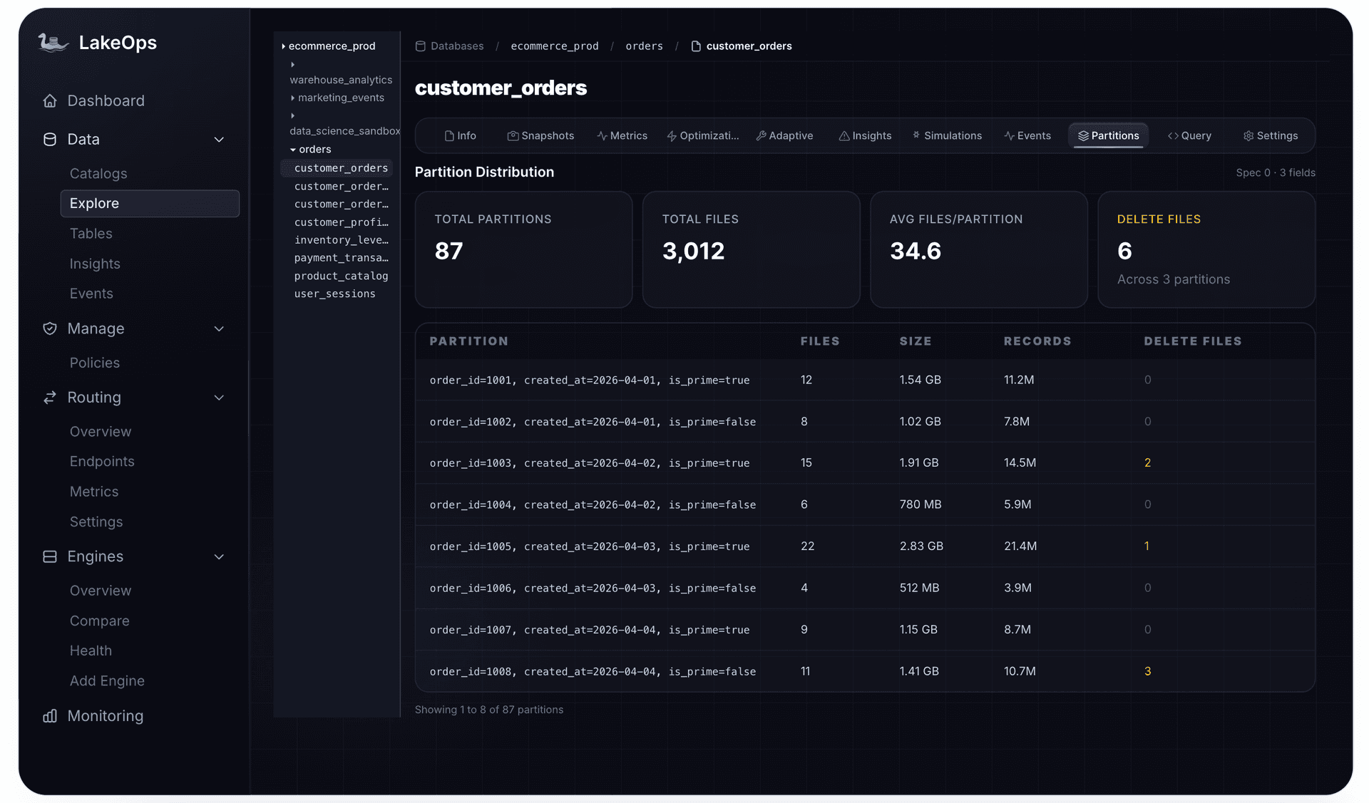
Without a control plane, tracking these signals means writing SQL queries against each table's metadata tables ($files, $snapshots, $manifests, $partitions), scheduling them in Airflow, parsing the results, applying classification logic, and repeating for every table in every catalog. Add a new catalog or a new table class, and the scripts need updating. It does not scale.

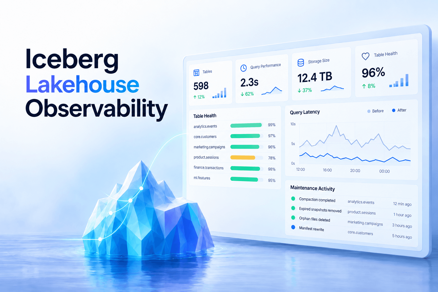
LakeOps computes all of these structural signals from catalog metadata continuously and automatically. Every commit to every table triggers a health reassessment. The result is a per-table structural profile — records, physical size, active and stale files, delete file counts, partition distribution, snapshot depth — that updates in real time without polling, without scheduled checks, and without compute cost.

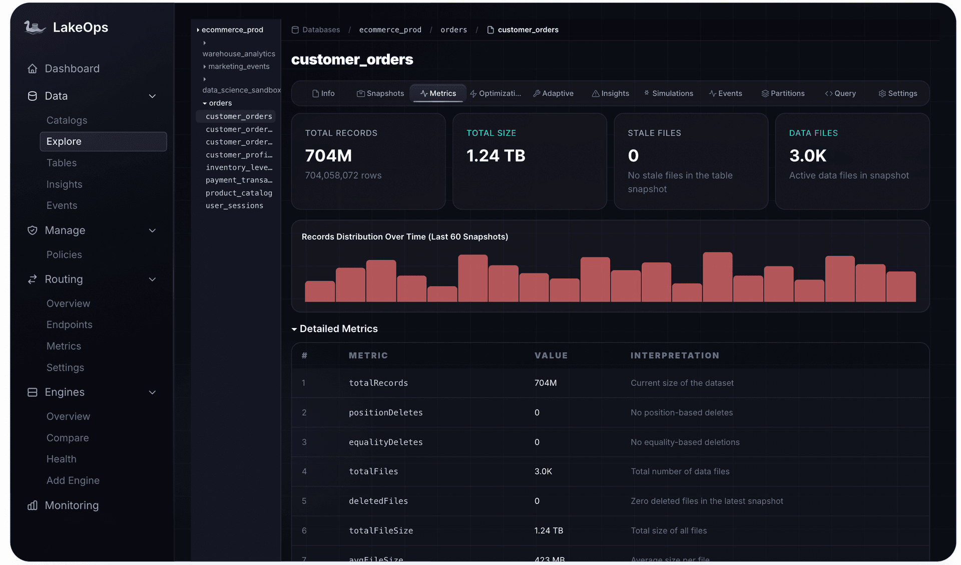
When an engineer investigates a slow query, this table profile shows whether the cause is structural (small files, manifest fragmentation, delete accumulation) or data-related (volume spike, partition skew) before they open a query plan. No SQL required. No scripts to maintain. LakeOps surfaces all of this through a unified Table Explorer for each table — metrics, partition distribution, snapshot history, per-table events, active insights, optimization status, layout simulations, and policy assignments — in a single view that serves as the operational hub for that table.

For a deep dive into each structural dimension with monitoring SQL queries and threshold guidance, see the data quality and table health guide.

Lake-wide health classification: turning hundreds of tables into a priority list

Tracking structural signals per table is necessary but insufficient at scale. With 200, 500, or 2,000 tables, the operational question is not what does each table look like — it is which tables need attention right now, and in what order.

This is where health classification transforms observability from a wall of metrics into an actionable system. Every table gets classified into one of three states:

• Critical — structural degradation severe enough to impact query performance or correctness. Average file size below 32 MB, delete-to-data ratio above 0.5, manifest ratio below 1:10, or snapshot retention exceeding policy by more than 5×. These tables need immediate remediation.
• Warning — degradation trends that will reach Critical without intervention. File sizes declining below 128 MB, delete ratios creeping above 0.1, snapshot depth drifting beyond policy. These tables need attention within the current maintenance cycle.
• Healthy — all structural signals within acceptable bounds. File sizes between 128–512 MB, manifests well-consolidated, snapshots within retention policy, sort order aligned with actual query patterns. These tables get zero maintenance compute — because they don't need it.

But classification at three levels is still too coarse for production operations. A single Critical table might have four independent issues at different severity levels. LakeOps implements a four-severity Insights model that provides issue-level granularity within each table:

• CRITICAL — immediate performance impact (85,000 small files in a hot partition, metadata corruption risk)
• HIGH — significant degradation requiring prompt action (4,200 pending position delete files, 12,000 un-expired snapshots)
• WARNING — emerging trends that will escalate without correction (sort order misaligned with dominant query predicates, file sizes declining below 128 MB)
• LOW — minor inefficiencies to address when convenient (12 orphan files consuming 340 MB, single partition with slight skew)

Each Insight surfaces the specific metric, its current value, the threshold violated, and the remediation action. CRITICAL and HIGH Insights trigger automated remediation. WARNING and LOW Insights surface for review without paging anyone. This distinction — page on correctness and availability, report on efficiency — is the difference between observability that drives operational sanity and monitoring that drives alert fatigue.

Classification must also be context-aware. A streaming events table receiving commits every 30 seconds with 500 small files per partition is in worse shape than a monthly reporting table with the same count — because the streaming table is queried thousands of times per day. Per-table policies that encode workload expectations (compaction frequency, target file size, acceptable delete ratio, snapshot retention) are essential for accurate classification. LakeOps applies these policies per table so a CDC table with aggressive write throughput is classified against different thresholds than a daily-batch dimension table.

The operational record: events, history, and accountability

Observability is not only about the current state of the lake — it is about the operational history that explains how it got there. When a table's health changes, when a maintenance operation runs, when a policy is applied — every one of these events must be logged with enough context to answer: what happened, when, why, and what was the impact?

This operational record serves three distinct purposes in a production lakehouse:

Debugging and root-cause analysis. When a query regression is reported on Thursday, the event trail shows that a compaction job ran on Wednesday that restructured the table's file layout. Did the new layout improve or degrade read patterns? Did the compaction exclude hot partitions that concurrent writers were updating? The answers are in the event log, with before-and-after metrics for every operation.

Compliance and audit readiness. Regulated industries need answers: what changed in this table, when, and who (or what) initiated it? Every maintenance operation — compaction, snapshot expiration, orphan cleanup, manifest rewriting — logged with start time, duration, files processed, bytes before and after, health score change, and outcome.

Operational review and optimization. Over time, the event trail reveals patterns: which tables generate the most maintenance work, which operations have the highest impact, whether maintenance frequency is adequate or excessive. This is the feedback loop that turns observability from a snapshot into a learning system.

Alongside the event trail, the snapshot explorer provides a complementary operational view: every snapshot for every table, with the ability to tag, branch, compare, and roll back. When a compaction job restructures a table and downstream queries behave differently, the snapshot history lets you inspect the exact state before and after — and restore the previous state in one action if needed. Time travel, branching, and rollback are not just features of the Iceberg format; they are operational observability surfaces that a production platform must expose.

Without this operational memory, maintenance is a black box. You know the lake was slow last month and it's faster now, but you cannot explain why — or predict what will happen next month. With it, every operational decision is traceable, every impact is measured, and every future plan is grounded in evidence.

Observability-driven adaptive maintenance: when seeing drives doing

The most powerful application of lakehouse observability is the maintenance loop it enables. In a traditional setup, maintenance is schedule-driven: a cron job runs compaction nightly on all tables, snapshot expiration weekly, orphan cleanup monthly. This approach has two problems. First, it wastes compute on tables that don't need it — a healthy table that hasn't changed gets compacted anyway. Second, it misses tables that need urgent attention — a high-throughput streaming table that degrades hourly waits until the nightly window. The next evolution of this pattern — self-healing pipelines powered by AI agents — uses observability signals to drive autonomous corrective actions across the entire lake.

Observability-driven maintenance replaces schedules with signals. The health classification layer identifies which tables need attention and ranks them by severity. The maintenance engine acts on that ranking, running the right operations in the right sequence on the right tables — and skipping everything else. This is especially critical for streaming tables: a Flink or Kafka-connected pipeline checkpointing every 30–60 seconds across hundreds of partitions can produce thousands of small files per hour. Fixed nightly maintenance is hours too late. Signal-driven maintenance responds within the cycle, before the file count compounds into a planning bottleneck.

The sequence matters more than most teams realize. Iceberg's maintenance operations have strict dependency relationships:

1. 1.Expire snapshots — removes old snapshots and dereferences data files they exclusively held
2. 2.Remove orphan files — cleans up files on storage that no snapshot references (only safe after expiration)
3. 3.Compact data files — merges small files into target-sized files, and resolves accumulated delete files by merging them into their corresponding data files (only efficient after expiration has removed files that compaction would otherwise needlessly rewrite)
4. 4.Rewrite manifests — consolidates fragmented manifests (only meaningful after compaction has stabilized the file set)
5. 5.Refresh statistics — updates Puffin statistics files that engines use for query planning (only accurate after compaction has finalized the file set)

Running these out of order wastes compute. Compacting before expiring snapshots rewrites files that expiration would have removed. Cleaning orphans before expiring snapshots misses orphans that expiration would create. The dependency chain must be respected per table, automatically, on every maintenance cycle. If you are managing this yourself, you are encoding these dependencies in Airflow DAGs, managing Spark cluster sizing per operation, handling OCC conflicts when maintenance collides with production writes, and hoping the scripts work correctly across hundreds of tables with different characteristics. It is the single largest source of platform engineering toil in production Iceberg deployments.

LakeOps runs this sequenced maintenance pipeline autonomously. The execution engine is built on Apache DataFusion in Rust — no JVM startup overhead, no garbage collection pauses, no cluster provisioning. Non-blocking commits ensure that concurrent readers and writers are never interrupted during maintenance. Operations complete on a purpose-built engine, not a repurposed Spark cluster, so maintenance compute cost is a fraction of the alternative.

The closed-loop measurement is what makes this adaptive rather than just automated. After every operation, the system measures outcomes: file count before vs. after, average file size improvement, planning latency delta, bytes reclaimed. These measurements feed back into future decisions. Tables where sort compaction produced large query acceleration get prioritized for sort maintenance. Tables where bin-pack sufficed skip unnecessary rewrites. The system improves with every cycle because it learns from its own observations. For a detailed walkthrough of autonomous maintenance operations and their production mechanics, see the dedicated guide.

Multi-engine observability: what no single engine can see

In a multi-engine lakehouse — the architecture Iceberg was designed for — the most valuable observability signals are invisible to any individual engine. Trino knows about its queries. Spark knows about its jobs. Flink knows about its checkpoints. No engine knows what all the other engines are doing to the same tables.

This multi-engine blind spot creates three classes of problems that only cross-engine observability can solve:

Conflicting access patterns. If 80% of Trino queries on a table filter on event_date and region, while 70% of Spark jobs filter on customer_id and product_category, the optimal sort order requires knowing both workloads. No single engine can determine it. Without cross-engine query telemetry, sort order decisions are made from one engine's perspective and may actively harm the other's performance.

Total cost attribution. The true cost of a table is the sum of all engine queries, all maintenance compute, and all storage — distributed across S3 billing, EMR/Dataproc usage, Trino cluster costs, and Athena per-query charges. No individual engine aggregates this. Per-table total cost of ownership requires collecting billing signals across every engine and service that touches each table.

Write-read coordination. Knowing that Flink commits to a table every 30 seconds while Trino federation queries hit it every 5 minutes allows maintenance to run between query cycles rather than during peak read windows. This coordination is invisible to either engine alone.

LakeOps collects query telemetry from every connected engine and correlates it per table. The result is a unified access profile: which engines read and write each table, which columns are filtered most frequently (across all engines), what the read amplification factor is per engine, and how query patterns shift over time. This profile drives optimization decisions that would be impossible from any single engine's perspective — and it feeds directly into query routing, where the right workload is directed to the right engine based on cost, latency, and table structure.

Cost observability: attributing spend to tables, not clusters

Lakehouse cost management is notoriously opaque. Object storage bills per bucket or prefix, not per table. Compute bills per cluster, not per query. Data transfer costs appear as line items with no table-level attribution. The result: most teams know their total lakehouse bill but cannot answer the question that matters — which tables are the most expensive to operate, and why?

Cost observability requires correlating three independent cost streams per table:

• Storage cost — active data files, but also retained snapshots pinning old data, orphan files from aborted writes, and metadata files. A table where 40% of storage cost comes from orphans has a cleanup problem, not a data growth problem.
• Query compute cost — attributed from each engine's billing model. A table where average query scan volume is 10× the result set has a layout problem that compaction and sort optimization would fix.
• Maintenance compute cost — the cost of keeping the table healthy. Over-maintained tables (compacting hourly when weekly suffices) waste compute. Under-maintained tables (never compacting a streaming table) waste far more in query compute downstream.

The highest-value signal is cost per query per table. A table where each query costs $0.50 because small files force full scans might cost $0.05 after compaction. Across 10,000 daily queries, that is $4,500 per day in unnecessary spend — invisible without per-table attribution. Most teams discover this waste only when the monthly bill arrives and someone asks why it doubled. A control plane surfaces it continuously, traces it to specific tables, and shows exactly which structural improvements would reduce it most — before the bill arrives.

Governance and policies: encoding standards at lake scale

Observability tells you the state of the lake. Governance tells the lake what state it should be in. Policies are the mechanism that connects the two — declarative rules that encode what "healthy" means for each table or class of tables, and what actions should be taken when health drifts outside acceptable bounds.

Without policies, every table is governed ad hoc — someone remembers to check it, someone writes a script, someone schedules a manual compaction. At 20 tables, this is inconvenient. At 200, it is untenable. At 2,000, it is a full-time job for a team.

Policies encode the operational intent: target file size, compaction strategy (bin-pack vs sort), snapshot retention period, orphan cleanup frequency, acceptable delete-to-data ratio, and the severity thresholds that trigger automated remediation. Different table classes get different policies — a streaming events table with aggressive write throughput needs different parameters than a quarterly finance snapshot.

The interplay between observability and governance is what creates a truly managed lakehouse. Observability detects that a table's file sizes are declining. Classification flags it as Warning. The policy for that table's class says: trigger sort compaction when average file size drops below 128 MB, targeting 512 MB output files, using the sort order derived from the top-3 filter columns across all engines. The maintenance engine executes. The event trail records the operation and its impact. The next health check verifies the table is back to Healthy. No human intervention. No ticket. No Slack message.

Layout intelligence: optimizing file organization from real query patterns

One of the most powerful applications of lakehouse observability is layout optimization — reorganizing how data is physically arranged within files to match how it is actually queried. This goes beyond basic compaction (merging small files) to sort optimization (ordering rows so that query predicates skip entire files) and partition strategy validation.

The insight driving layout intelligence is simple: Parquet files store per-row-group min/max statistics. If a query filters on event_date, and the data is sorted by event_date, most row groups have non-overlapping ranges and the engine skips 95% of the data without reading it. If the data is sorted by customer_id instead, every row group's event_date range overlaps with the filter, and nothing gets skipped.

The challenge is determining the optimal sort order when multiple engines query the same table with different predicates. This requires aggregating query telemetry across all engines, weighting by query frequency and cost, and computing the sort key that maximizes data skipping across the combined workload.

LakeOps performs this analysis continuously. It collects query patterns from every engine, identifies the optimal sort configuration per table, and validates it through layout simulations run on Iceberg branches — isolated from production. Only after a simulation confirms improvement does the change get committed. This is observability applied to its highest-leverage use case: making every query faster by aligning physical data layout with actual access patterns.

Connected catalogs: the foundation of lake-wide visibility

Observability at lake scale starts with connectivity. A production Iceberg lakehouse typically spans multiple catalogs — AWS Glue for some tables, a REST catalog (Polaris, Nessie, Gravitino) for others, S3 Tables for managed tables. Each catalog manages its own set of tables. Without a system that connects to all of them, observability is fragmented by design.

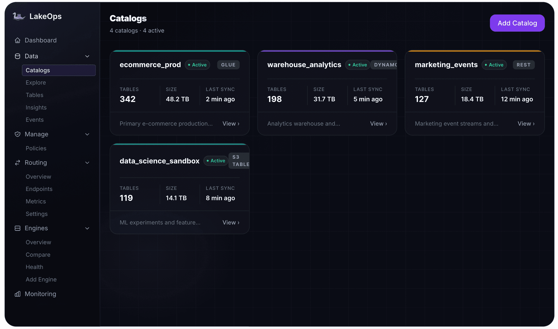
LakeOps' catalog integration connects to every major Iceberg catalog through standard APIs. Once connected, every table in every namespace in every catalog appears in the unified management interface — with health classification, structural metrics, operational history, and policy enforcement applied uniformly. The lake stops being a collection of isolated catalogs and becomes a single observable entity.

The executive view: lake-wide operational health at a glance

Platform engineering leadership needs a different lens on observability than individual data engineers. The executive view answers two questions: Is the lake healthy? and Is the investment in lakehouse operations paying off?

This requires aggregated, trend-based metrics: total tables under management, tables by health state (with trends), total maintenance operations run, average query acceleration achieved from optimization, cumulative cost savings from orphan cleanup and scan reduction, total CPU hours and storage reduced, and month-over-month trajectories.

These aggregated metrics serve a purpose beyond reporting. They validate the observability system itself. If total tables classified as Critical is rising month over month, either the lake is growing faster than maintenance can keep up, or the classification thresholds need recalibration. If cost savings flatten, either the low-hanging fruit has been captured and optimization should shift to layout intelligence, or new cost vectors (cross-region reads, metadata API costs) need attribution. The executive view is observability applied to the observability system.

From blind to managed: implementing lakehouse observability

Building a complete observability stack does not require implementing every layer simultaneously. The practical path has three stages, each delivering immediate value while building toward full coverage.

Stage 1: Connect and classify

Connect your catalogs and engines. Compute structural health metrics for every table from existing metadata — no agents to install, no data to instrument. Classify every table by health state. This stage alone transforms the operational posture: you go from we think most tables are probably fine to we know exactly which 47 tables are degraded and which 12 are critical.

The time investment is minimal. LakeOps connects to most catalogs and engines in under ten minutes. The health classification runs continuously once connected. Stage 1 delivers the foundation: visibility across the entire lake.

Stage 2: Automate maintenance and track operations

With classification in place, enable adaptive maintenance for Critical and Warning tables. Run the sequenced pipeline (expire → clean → compact → rewrite → refresh statistics) automatically, driven by health signals. Log every operation in the event trail. Measure before-and-after impact.

This stage closes the loop from observation to action. Tables that were degrading for weeks get remediated in hours. The event trail provides the operational history that debugging and compliance require. The lake starts maintaining itself.

Stage 3: Optimize and govern

With health stable, move to optimization: enable cross-engine query telemetry, apply sort optimization from access patterns, implement per-table policies for governance, and build cost attribution per table. For teams building automation, LakeOps exposes every observability signal through a REST API and an MCP server — enabling AI agents and CI/CD pipelines to query lake health, triage critical tables, analyze policy gaps, and trigger maintenance programmatically. To understand how AI agents can monitor data quality on Iceberg using these observability signals, see the dedicated guide. This is where the lake moves from maintained to managed — and where the ROI of observability compounds, because every optimization is grounded in real signals.

Observability is the foundation, not a feature

Every operational capability in a managed data lakehouse depends on observability. Maintenance needs health signals to know what to fix. Compaction needs query patterns to choose the right strategy. Cost optimization needs per-table attribution to identify waste. Governance needs classification to enforce policies. Query routing needs engine telemetry to direct workloads. Without observability, every one of these capabilities is either manual, blind, or both.

The teams running production Iceberg lakehouses at scale — hundreds of tables, multiple engines, petabytes of data — have learned this through experience. The table format gives you open, vendor-neutral storage. Observability gives you the ability to understand and maintain it. And a control plane like LakeOps gives you both at lake scale, continuously, without the operational overhead consuming your platform team.

The difference between a data lake and a managed data lakehouse is not the table format. It is not the catalog. It is not the engines. It is whether you can see what is happening across every table, every engine, and every dollar of spend — and whether that visibility drives automated action. That is observability. And it is the first thing you should implement after your first table lands. For teams building toward AI-native architectures, see how to make your Iceberg lakehouse AI-ready — ensuring observability, governance, and data layout support both human and AI consumers.