
A data lakehouse is a warehouse-grade transactional layer built directly on object storage. Files live in S3, GCS, or ADLS; an open table format lets many engines read and write the same data correctly; a catalog makes every engine agree on the current version. You get ACID commits, schema evolution, and time travel without copying data into a proprietary system.
That is the architecture in one paragraph. Building one that still performs at 2,000 tables is a different problem — and it is mostly not about the parts you choose. A working lakehouse has five layers: object storage, a table format, a catalog, query engines, and an operational layer that keeps tables healthy. The first four are increasingly commodity. The fifth is the one teams discover months after going live, when queries that took two seconds take forty and nobody can say which table is responsible.
This guide covers all five: what each does, the mechanism underneath, and what breaks as the lake grows. Two companion pieces work backwards from how large engineering organizations solved the operational layer — how Netflix built an intelligent lakehouse and how Google structures an open lakehouse for performance. This is the ground-up version of the same architecture.
The five layers, and the one most teams skip
Each layer has one job, and each depends on the one below it:
| Layer | Job | Common implementations | What goes wrong |
|---|---|---|---|
| Object storage | Durable, cheap bytes | S3, GCS, ADLS | Request cost and per-file overhead scale with file count |
| Table format | Turn files into a transactional table | Apache Iceberg | Metadata grows faster than data; delete files accumulate |
| Catalog | Hold the current table pointer; authorize access | Glue, Polaris, Nessie, Lakekeeper, S3 Tables | Single point of failure for every read and write |
| Query engines | Execute SQL and jobs | Trino, Spark, Flink, DuckDB, Snowflake, Athena | Each engine commits independently; conflicts and skew |
| Control plane | Keep every table healthy, laid out, and governed | Usually nothing, or scripts | Nobody owns it, so table health degrades silently |
The first four layers are what you install. The fifth is what you operate, and operating is where the recurring cost lives. Iceberg tables degrade under normal, correct use. Streaming ingest produces small files, because commit frequency trades off against file size. Every commit adds a snapshot until metadata reads get expensive. Every update writes delete files readers must reconcile until something rewrites them. Manifests multiply and planning slows. This is not misuse — it is the arithmetic of append-oriented writes against an immutable file layout.
The remedies are documented: rewrite_data_files, expire_snapshots, remove_orphan_files, rewrite_manifests. Running them was never the hard part. The hard part is knowing that orders_fact needs compaction today, clickstream_raw needs it hourly, dim_currency should be skipped, compacting the partition your streaming writer is appending to will lose a commit race, and sorting by customer_id helps nothing if every query filters on event_date.
At 20 tables an engineer holds that in their head. At 200 the DAG encoding it is a second system with its own failures and thresholds nobody remembers choosing. At 2,000 across several catalogs and engines, most of the lake is unmanaged — the team finds out through a latency regression or a cloud bill.
What a control plane is, and why it belongs in the architecture
A control plane is the operational intelligence layer for a lakehouse. It sits above the stack you already have — catalogs, Iceberg tables, query engines — and runs the loop none of them provides as a single system: observe every table, decide what each one needs, execute it in the right order, and verify the result. LakeOps is a control plane in this sense: observability, governance, and control while continuously maintaining and optimizing every Iceberg table and query engine for performance and cost.
Four properties define the category:
- 1.It is not a catalog, an engine, or a storage layer. It does not replace Spark, Trino, Glue, Polaris, or S3, and it does not own your data.
- 2.It attaches through metadata, not migration. It reads Iceberg metadata through standard catalog APIs — no data copy, no pipeline rewrite, no format change. Connecting one takes about ten minutes, and your data never leaves your cloud account.
- 3.It sees the whole lake, across engines. Per-table scripts and single-vendor optimizers cannot rank 2,000 tables or observe what five engines are querying.
- 4.It closes a loop. A cron job runs what you told it to; a control plane decides what to run from current evidence and gets better as that evidence accumulates.
That loop has four stages:
- Sense — Iceberg metadata and cross-engine query telemetry: file count and size, manifest depth, snapshot accumulation, delete-file ratio, partition skew, write velocity, and which columns queries filter, join, and group on.
- Plan — classify each table, rank by severity so the worst-degraded go first, and sequence operations so each step's output is the next step's clean input.
- Optimize — run maintenance and layout changes on an engine built for that job rather than a general-purpose cluster.
- Learn — measure the outcome and feed it back, so sort orders, cadence, and routing improve on the next pass.

Treating this as a first-class layer rather than a backlog item is the biggest difference between a lakehouse that holds up and one that quietly rots. Each section below builds a layer, then what the control plane contributes to that layer and how.
Layer 1: object storage and the economics of file layout
S3, GCS, and ADLS are interchangeable for lakehouse purposes. The fact that matters is that object storage prices requests, not just bytes — and Iceberg turns your table layout into a request pattern. A query scanning 40,000 small files issues roughly 40,000 GET requests plus the metadata reads to find them. The same data in 400 well-sized files issues about 400. Bytes scanned may be identical; the request bill and per-file open overhead differ by two orders of magnitude.
Practical targets:
- 128–512 MB per data file for analytical tables. AWS S3 Tables defaults to 512 MB with a 64 MB floor.
- Smaller files are legitimate for point-lookup tables, where you read one row rather than scan a range.
- One prefix per table, with unique table locations enabled. Iceberg 1.11 appends a UUID to table paths, closing a data-loss scenario where
remove_orphan_fileson a renamed table could delete files still referenced elsewhere.
Two storage decisions interact badly with automation:
Storage-class tiering can silently defeat maintenance. On S3 Tables with Intelligent-Tiering, compaction runs only on files in the Frequent Access tier. Files that have aged colder are not compacted — and deletes against cold data create delete files that become eligible only once the data files are accessed and move back. On an infrequently-read table, merge-on-read overhead can accumulate under a system you believed was maintaining it.
Lifecycle rules do not understand Iceberg. An S3 lifecycle policy that expires objects after N days will delete data files a live snapshot still references, corrupting the table. Snapshot expiry belongs to Iceberg, not the bucket. Use lifecycle rules for storage-class transitions, never deletion.
Layer 2: Apache Iceberg and how a table actually works
The table format is what makes a directory of Parquet files behave like a database table. Its structure is worth knowing — every performance and cost problem later in this guide follows from it.
Iceberg maintains a tree, and a read walks it top-down:
- 1.The catalog holds a pointer to the current metadata file (
vN.metadata.json) — the atomicity mechanism for the whole table. - 2.The metadata file holds schema, partition spec, sort order, properties, and the snapshot list.
- 3.A snapshot represents the table at one point in time and points to a manifest list.
- 4.The manifest list points to manifest files, each with partition-range summaries so whole manifests can be skipped at planning time.
- 5.A manifest file lists data files with per-column min/max values, null counts, and row counts.
- 6.Data files are Parquet (or ORC/Avro), divided into row groups with their own statistics.
Two consequences follow directly:
Writes are optimistic, not locked. A writer reads current metadata, writes new data files, builds new metadata, then asks the catalog to swap the pointer only if it still points where the writer started. If another writer committed first, the swap fails and the writer retries. That is what lets Spark, Trino, and Flink write the same table — and why maintenance jobs lose races against active writers.
Query planning reads metadata, and metadata grows. Before reading a byte of data, an engine walks manifests to decide which files it needs, and every commit adds to that structure. A table with 487 manifests spends real time planning before it starts work; consolidating to a dozen cuts planner latency from seconds to a fraction of one. Metadata maintenance is a performance feature.
Format version 3 is the sensible default now
Iceberg V3 was approved in late 2025 and rolled out across engines through 2026. The most consequential change is the delete path.
In V2, a row-level delete was recorded in a position delete file naming a data file path and row position. Readers had to collect every applicable delete file and reconcile them against data files — a join against a delete index at read time. Under CDC or update-heavy workloads these proliferate, and every read pays until compaction rewrites them away.
V3 replaces this with deletion vectors: each data file gets at most one paired vector, a Roaring bitmap in a Puffin sidecar marking deleted row positions. A reader scanning orders-0042.parquet consults that file's own bitmap — no global delete index to join against. This collapses the read path, shrinks metadata, and removes most of the write amplification that made frequent updates and GDPR-style deletes expensive.
The rest of V3:
- Row lineage is mandatory — every new row carries
_row_idand_last_updated_sequence_number, giving CDC without a separate change log. Limitation: lineage is not tracked for rows updated via equality deletes, because the engine never reads the existing row. variantstores semi-structured data with per-row schema flexibility.geometryandgeography, with bounding-box types and anINTERSECTSpredicate, make spatial pruning native.- Column defaults, multi-argument transforms, and nanosecond timestamps remove long-standing workarounds.
Upgrading to format-version = 3 is effectively irreversible, and every reader must support V3:
| Engine / platform | V3 status |
|---|---|
| Spark 4.0+ / Iceberg 1.10+ | Most complete open-source support |
| AWS (EMR 7.12+, Glue, S3 Tables) | Deletion vectors and row lineage |
| Snowflake | GA — deletion vectors, lineage, variant, geospatial, defaults |
| Databricks (Runtime 18.0+) | Preview; no defaults, ns timestamps, or multi-arg transforms |
| Flink 2.1 / Iceberg 1.11 | Deletion vectors and variant; lineage through RewriteDataFiles |
| Open-source Trino | Not yet; Starburst supports it |
| BigQuery | Reads deletion vectors; cannot write V3 |
| PyIceberg | Reads V3; writes limited |
The rule: inventory every reader — including the BI tool, the notebook, and the Python job nobody owns — before flipping the version. Open-source Trino lagging is the most common blocker, because Trino is often the serving engine in exactly the architectures that most want deletion vectors.
Layer 3: the catalog is the atomicity and authorization boundary
The catalog's job is small and critical: hold the pointer to each table's current metadata file and swap it atomically on commit. That store is the correctness boundary for the lakehouse. And because engines get storage access through the catalog, it is also the authorization boundary.
That makes the catalog the highest-availability component in the architecture. A catalog outage is not degraded performance — queries, writes, and scheduled jobs fail together. Single-replica is a development pattern, not a production one.
The Iceberg REST Catalog specification has won as the interface. Glue, Polaris, Nessie, Gravitino, Lakekeeper, and S3 Tables are implementations behind one protocol, which makes catalog choice operational rather than architectural lock-in. For deploying one — persistence, realm bootstrap, token signing, and the failure modes the quickstart omits — the Apache Polaris guide covers it, and the catalog comparison weighs the options.
Three protocol capabilities worth designing around:
Credential vending. Rather than distributing long-lived cloud keys to every engine, the catalog issues short-lived, table-scoped storage credentials per request. This is the largest security improvement available in a lakehouse and the main reason to prefer a REST catalog over a Hive Metastore. Caveat on federation: when Polaris federates to a remote Iceberg REST catalog it does not forward access-delegation headers — it mints credentials locally, so the federating deployment needs its own storage configuration.
Server-side scan planning. Historically every client fetched manifests itself to work out which files to read. A REST catalog can now plan server-side: the client POSTs a predicate to /v1/{prefix}/namespaces/{namespace}/tables/{table}/plan and receives file scan tasks, inline or via a plan-id it polls. Iceberg 1.11 extended this to incremental scans and metadata tables. Driver memory pressure drops, and planning optimizations become a catalog-side concern.
Idempotency and freshness. An Idempotency-Key header on mutating operations means a retried commit cannot execute twice. ETag-based loading lets a server answer 304 Not Modified instead of resending metadata, and lets a client detect a concurrent write between its load and its commit.
How a control plane attaches here
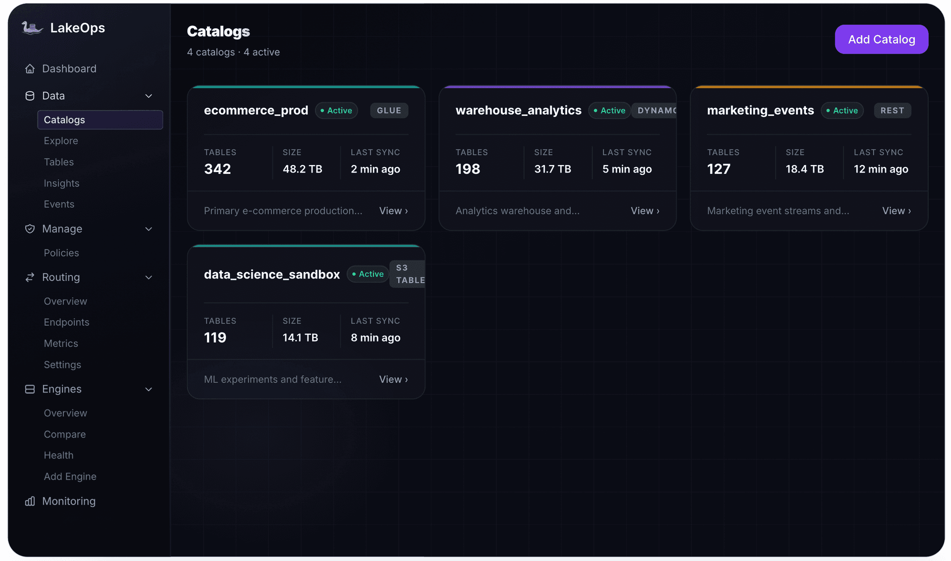
What it does: discovers every namespace and table across every connected catalog, then reads Iceberg metadata continuously to build a health picture of the whole lake.
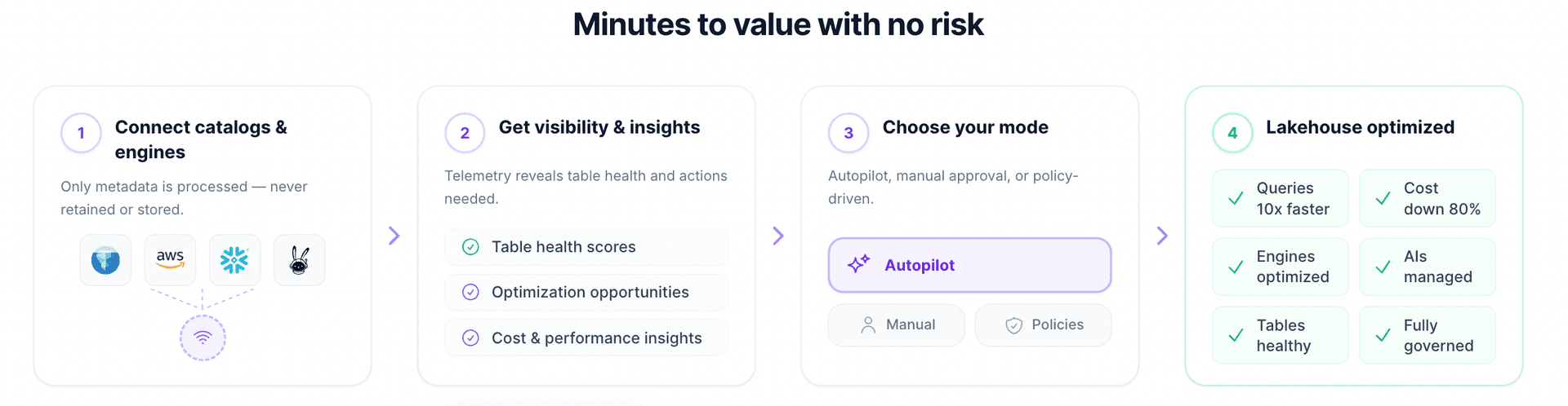
How it does it: through the same REST catalog and Iceberg metadata APIs your engines use. LakeOps connects to AWS Glue, Apache Polaris, Nessie, Gravitino, Lakekeeper, S3 Tables, and any REST-compatible catalog. No agents, no pipeline changes, no SQL to get started — only metadata is processed, and it is not retained. Connect once and every table is discovered automatically. The managed lakehouse overview covers what begins running on connection.
Because the control plane reads metadata rather than proxying queries, it is not in the critical path. Engines keep talking to the catalog directly. If the control plane is unavailable, maintenance pauses — queries do not.
Layer 4: the engine fleet
The architectural payoff is that storage and compute decouple: one physical copy of the data, many engines. In practice that means picking an engine per workload shape rather than per organization.
| Engine | Best at | Watch out for |
|---|---|---|
| Spark | Large ETL, shuffles, backfills, maintenance | Cluster startup, JVM GC, OOM on large rewrites |
| Trino | Interactive SQL, federated joins, BI | Memory-bound on huge joins; V3 support lags |
| Flink | Streaming ingest and CDC | Small-file production; checkpoint tuning |
| DuckDB | Single-node ad hoc, point lookups | Not for multi-TB shuffles |
| Snowflake / Athena | Governed SQL, serverless bursts | Highest per-query cost |
| StarRocks / ClickHouse | Low-latency aggregations | Another system to operate |
The engine question that matters most is eligibility: what determines whether a query can run on the cheap engine? Mostly table layout. A point lookup against a well-sorted table with lean manifests can be answered by a small engine reading a handful of files. The same query against a fragmented table with thousands of small files needs a distributed engine to brute-force it. Layout quality sets the floor on your minimum viable engine — a cost lever, not only a latency lever.
Coordination problems:
- Commit conflicts. Concurrent writers — including maintenance jobs — lose optimistic-concurrency races and must retry. Every Iceberg writer needs retry logic.
- Uneven V3 support. A table cannot be V3 if one reader cannot read V3. The fleet's capability is the intersection, not the union.
- Uneven statistics use. Engines differ in how aggressively they use Puffin statistics and min/max pruning, so one layout yields different skipping across the fleet.
- Uneven write behavior. From Iceberg 1.7.0,
WRITE ORDERED BYpreserveswrite.distribution-modewhile adding task-level sorting; before 1.7.0 it silently set it tonone. Mixed-version writers can produce different layouts from identical DDL.

The control plane as the multi-engine layer
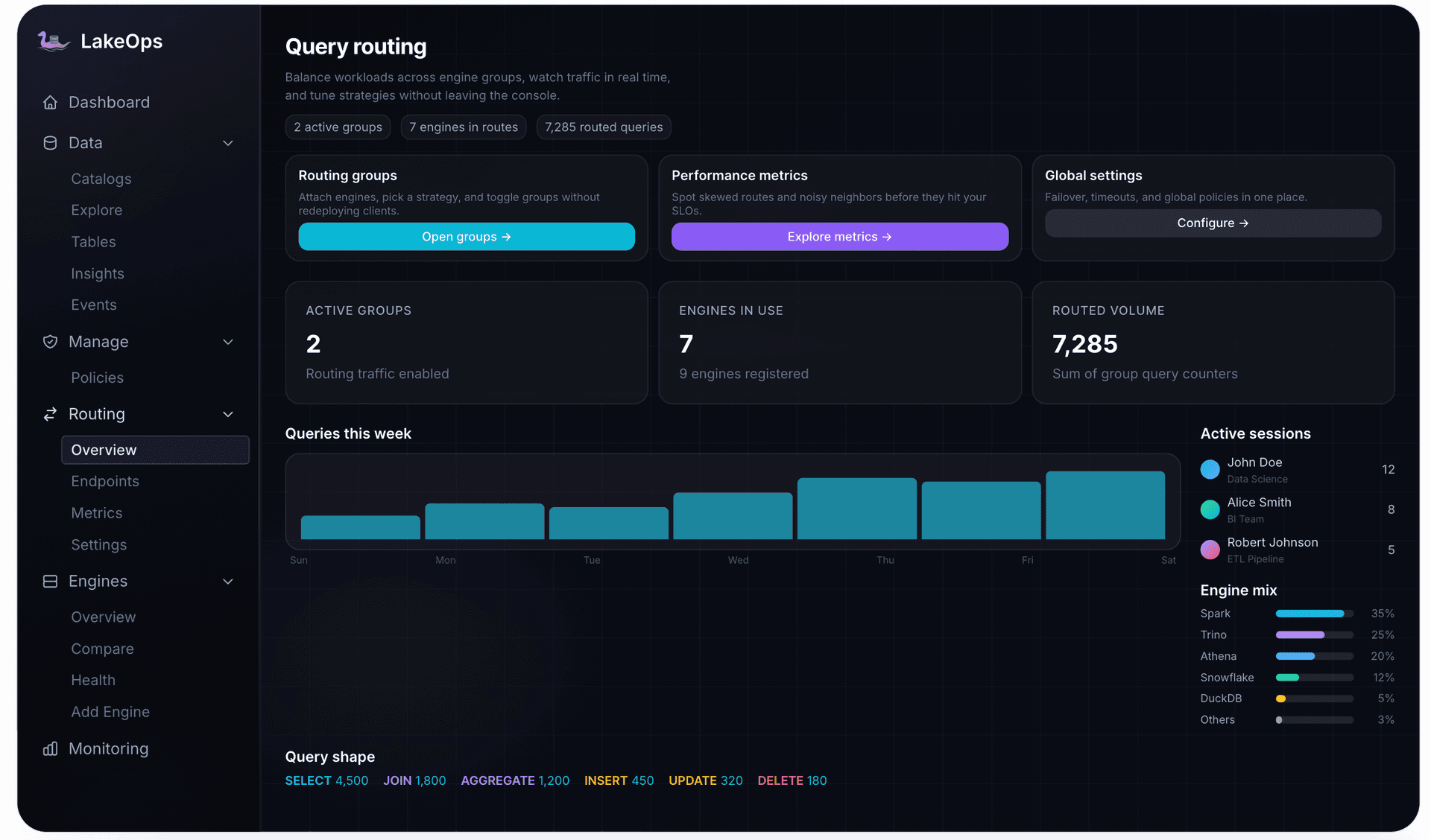
What it does: presents one SQL endpoint and dispatches each query to the engine that best fits it, while collecting unified telemetry across the fleet.
How it does it: LakeOps routes on an explicit strategy per routing group — latency, cost, or throughput — with groups organized by workload (analytics, BI, ETL, reports) rather than by team, each with its own endpoint, concurrency limit, and overflow queuing. It fails over when an engine's health degrades below threshold. The routing layer is QueryFlux, an open-source Rust SQL proxy speaking Trino HTTP, PostgreSQL wire, MySQL wire, and Arrow Flight SQL, translating dialects at about 0.35 ms p50. Because the endpoint is stable, you can add or swap engines without changing application code.
The compounding effect: as layout improves, more queries become eligible for cheaper engines, so routing decisions get better as maintenance does. Published benchmarks put point lookups at 0.5s on DuckDB against 2.3s on Athena for the same query, and workload-aware dispatch at up to 56% lower query spend. The multi-engine routing guide and the query routing page cover how to stage it.
The pruning stack: why lakehouse queries get slow
Most lakehouse performance problems are pruning problems, and most discussions collapse four distinct mechanisms into one word. They fail separately.
1. Partition pruning (coarse). The Iceberg partition spec with hidden transforms — year, month, day, hour, bucket, truncate, identity — determines which file groups can be ignored entirely. Partition evolution lets the spec change without rewriting history. The classic failure is over-partitioning: hour granularity on a moderate table produces thousands of tiny partitions and a metadata problem worse than the scan problem it solved.
2. File pruning via sort order, also called linear clustering (fine). Rewriting data so rows with nearby key values land in the same files tightens per-file min/max statistics, letting engines skip whole files. This is the layer most teams are missing, and where a critical asymmetry lives: a linear sort helps the leading column enormously and progressively less for each subsequent one. Sorting by (customer_id, event_date) prunes customer_id excellently and event_date alone poorly.
3. Z-order, or multi-dimensional clustering. Bit-interleaving across columns produces a space-filling curve so two to four columns all prune reasonably well, at the cost of none pruning as well as a leading sort column would. Right when several filter columns matter equally; wrong past about four, where the benefit dilutes toward no clustering.
4. Row-group pruning inside Parquet, plus file sizing and statistics. Row-group statistics allow sub-file skipping, which only helps if data inside the file is clustered. File size determines request count; manifest count, snapshot depth, delete-file burden, and Puffin freshness determine how expensive it is to even plan the scan.
Two statements worth keeping distinct:
Binpack compaction fixes file count. It does not cluster rows. Binpack merges small files by size alone: fewer, larger files with wide min/max ranges, so file pruning still fails. Tables get "compacted" on a schedule for months and queries never speed up.
"Cluster" means three different things. A clustering strategy is a sort order; file sizes grouping around the target is file-size distribution; a Spark cluster is compute. Databricks Liquid Clustering, BigQuery clustering, and Snowflake micro-partitions are not Iceberg sort order — compare, do not equate.
The control plane as the layout engine
Choosing a sort order is the highest-leverage decision in this stack and the one with the worst available information. A sort order declared at table-create time encodes a hypothesis about access patterns. Six months later the dashboards have changed, the hypothesis is stale, and nothing in the table tells you so. Managed compaction services apply whatever sort order you declared — choosing the right one is out of scope.
What it does: derives clustering keys from the queries your engines actually run, validates them before touching production, and executes the rewrite on a purpose-built engine.
How it does it: three mechanisms.
Query-aware key selection. LakeOps collects WHERE, JOIN, and GROUP BY column frequency from every connected engine — Trino, Spark, Snowflake, Athena, DuckDB — and ranks candidate sort columns by observed access. A representative profile: customer_id filtered in 89% of queries, event_date in 76%, product_id joined in 64%. That is a derived answer, not an opinion.
Layout simulation before rewriting. Candidate strategies run on an Iceberg branch, replaying production queries against baseline and candidate layouts. Published output shows sorting by event_date, region at roughly 8.3x with 62% less scanned, against customer_id, event_date at roughly 12.4x with 76% less scanned — same table, different outcome. Changing clustering rewrites files and is hard to undo.
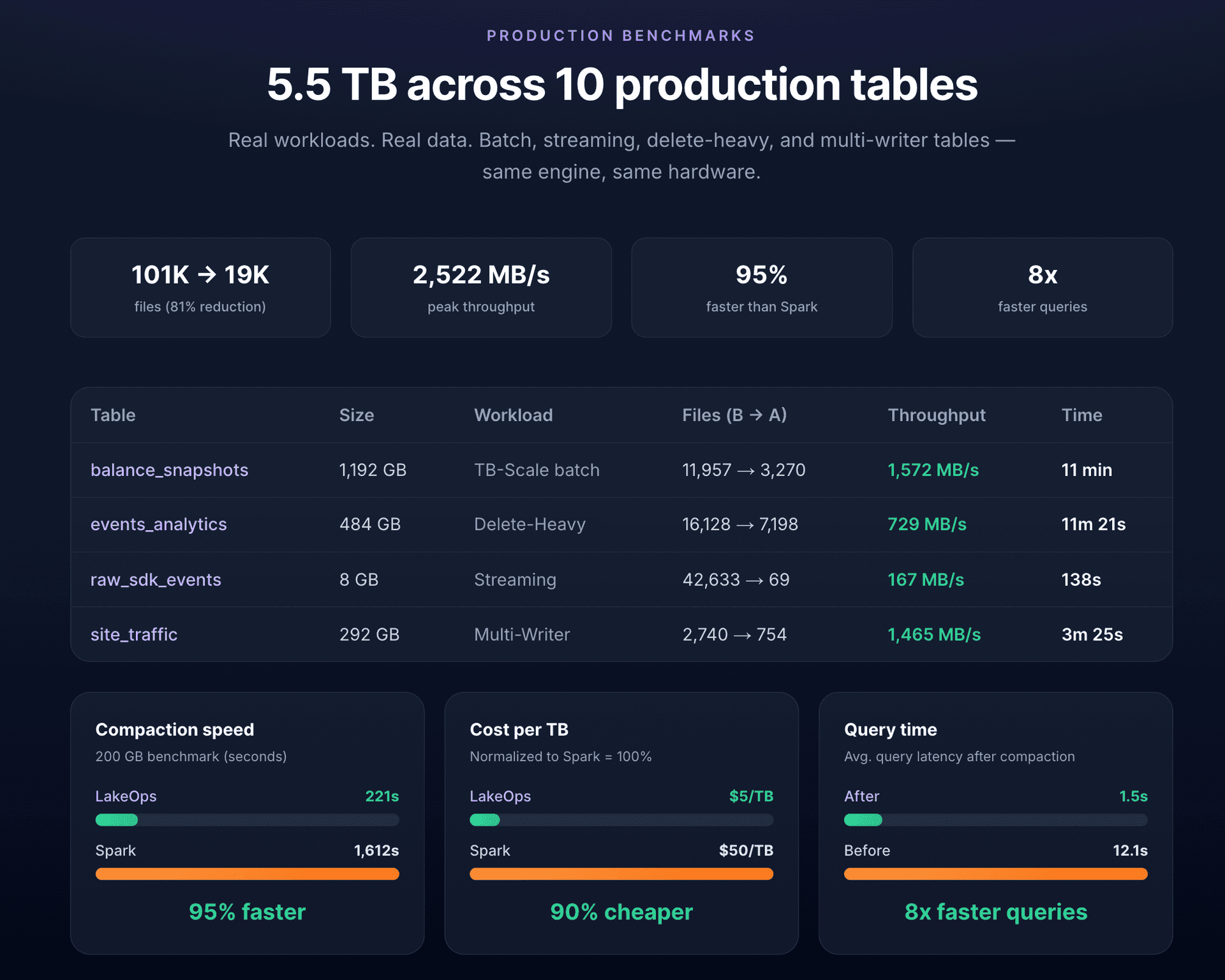
A compaction engine suited to the job. Compaction is a narrow, I/O-bound read-merge-write. Running it on a general-purpose cluster means JVM overhead, GC pauses, OOM risk, and a cluster to provision. LakeOps runs it on a Rust engine built on Apache DataFusion — zero-copy Arrow, bounded memory with disk spill, lock-free parallelism. On a published 200 GB / 600M-row binpack at the same target file size: 221 seconds at 2,522 MB/s, against 1,612 seconds on Spark and 6,300 on S3 Tables — roughly 95% faster than Spark at about a tenth of the cost per terabyte. A 1.2 TB table that exhausted Spark's heap completes in about 11 minutes. Deletes are resolved in the same pass, and Puffin statistics refreshed so engines plan against the new layout.

When binpack, sort, and Z-order each win: the compaction strategies guide and the query-aware compaction page.
Layer 5: the operational loop, and why order matters
Four procedures keep an Iceberg table healthy. They are not independent, and running them in the wrong order wastes most of the work. The chain is expire → compact → clean → rewrite:
- Expire snapshots first. Old snapshots pin old data files. Compacting before expiring means the rewritten-away files stay referenced and nothing is reclaimed.
- Compact second, now that the file set reflects live data only.
- Remove orphan files third, because compaction itself produces orphans — files written by a rewrite that then failed to commit are unreferenced by definition.
- Rewrite manifests last, so consolidation reflects the final file set rather than an intermediate one.
Any other sequence operates on stale input or is immediately invalidated by the next. This ordering is a property of Iceberg's design, not a vendor opinion.
1-- 1. Expire first: old snapshots pin old files.2CALL catalog.system.expire_snapshots(3 table => 'db.orders_fact',4 older_than => TIMESTAMP '2026-09-01 00:00:00',5 retain_last => 106);7 8-- 2. Compact, sorted by observed filter columns.9ALTER TABLE catalog.db.orders_fact WRITE ORDERED BY customer_id, event_date;10 11CALL catalog.system.rewrite_data_files(12 table => 'db.orders_fact',13 strategy => 'sort',14 sort_order => 'customer_id ASC NULLS LAST, event_date ASC NULLS LAST',15 options => map(16 'target-file-size-bytes', '268435456',17 'min-input-files', '5',18 'delete-file-threshold', '2',19 'partial-progress.enabled', 'true',20 'partial-progress.max-commits', '10',21 'max-concurrent-file-group-rewrites', '4'22 )23);24 25-- 3. Clean orphans this rewrite just produced.26CALL catalog.system.remove_orphan_files(27 table => 'db.orders_fact',28 older_than => TIMESTAMP '2026-09-18 00:00:00'29);30 31-- 4. Rewrite manifests last, against the final file set.32CALL catalog.system.rewrite_manifests(table => 'db.orders_fact');The parameters that decide whether this helps:
partial-progress.enabledcommits file groups incrementally — on a large table, the difference between keeping progress after a failure and losing hours of work.min-input-filesskips groups that are already fine.delete-file-thresholdforces a rewrite where delete files have accumulated even if file sizes look acceptable.max-concurrent-file-group-rewritesis the throughput/contention dial. Higher finishes sooner and loses more commit races against active writers.
remove_orphan_files is the one that can destroy data. It deletes files in storage that metadata does not reference. Three ways that goes wrong: an aggressive older_than deletes files an in-flight write has staged but not committed; a location shared by more than one table deletes the other table's files; and path-scheme mismatches (s3:// versus s3a://) can make referenced files look unreferenced. Keep a multi-day safety window and one location per table.
This does not stay a cron job because the right answer per table changes. A streaming table may need hourly compaction, a daily batch table daily, a slowly-changing dimension effectively never. A schedule that ignores this either under-maintains hot tables or burns compute rewriting cold ones — and both failures are invisible until you go looking.
The control plane as the maintenance system
What it does: decides per table, per cycle, which of the four operations are needed, in what order, and at what cadence — then runs them safely alongside active writers.
How it does it: LakeOps monitors file count, small-file ratio, delete-file depth, snapshot age, manifest bloat, and write velocity per table, adapting cadence: streaming tables hourly, batch tables daily, healthy tables skipped. Operations follow the dependency order above automatically. Snapshot expiry is concurrency-safe — it will not expire a snapshot a running query still references — and retention is configurable from 3 to 90 days. Orphan removal uses a set-difference scan against live metadata with a default seven-day safety window, typically reclaiming 20–40% of storage on a lake that has never had it run.
Effects most schedules never reach: manifests from 487 to 12, planner latency from 3.4s to 1.3s, 97.5% fewer metadata reads; snapshots from 154 to 24 with metadata 84% smaller; delete files resolved so a 1.8-second read penalty goes to zero; data files from 970 to 87 with 62% fewer S3 GET requests. The table maintenance page details each operation, and automating Iceberg table maintenance covers the progression from DAGs to autonomous operation.


Snapshots, time travel, and retention
Snapshot history is what makes a lakehouse debuggable, and where retention has the most direct cost consequence. Every commit creates a snapshot, and each snapshot pins the data files it references. Three capabilities worth designing around:
- Time travel.
SELECT ... FOR TIMESTAMP AS OForFOR VERSION AS OFanswers "what did this table look like when that report ran?" - Rollback.
rollback_to_snapshotreverts a bad write atomically, without a restore from backup. - Branches and tags. Named refs let you stage a write, validate it, then fast-forward — the same mechanism layout simulation uses.
Retention is a direct cost dial. Ninety days of snapshots on a high-velocity table can pin several times the live data footprint. Retention generous enough for the auditor is expensive on a streaming table and free on a monthly dimension, so a single lake-wide number is always wrong somewhere. Setting it per table is correct — and needs to be expressed as policy rather than remembered.
Observability: measure before you automate
You cannot operate what you cannot see, and the default state of a lakehouse is that table health is invisible. Iceberg exposes the raw material through metadata tables — files, snapshots, manifests, partitions, history. The problem is not access. Answering "which of my 2,000 tables is worst right now?" means joining several metadata tables across every catalog, repeatedly, and knowing what threshold constitutes bad.
The signals that matter:
- File count and size distribution — fragmentation. A long tail of small files is the most common cause of slow scans.
- Average file size against target — whether compaction is keeping up with ingest.
- Manifest count and depth — planning overhead, paid before any data is read.
- Snapshot count and age — storage pinned by history.
- Delete-file ratio — merge-on-read overhead on every read.
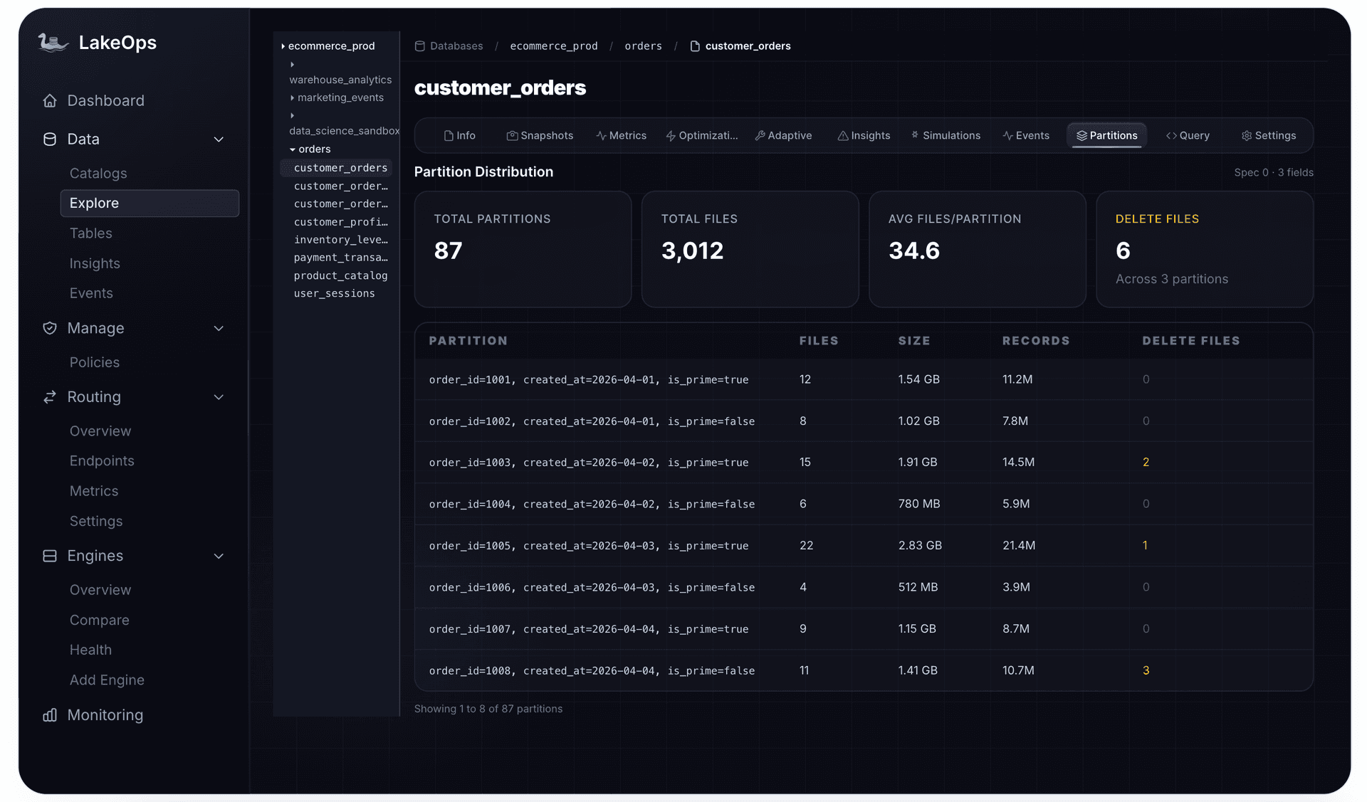
- Partition skew — one partition with 87 files where others have 12 sets query latency.
- Sort-order drift — the declared clustering no longer matches what queries filter on.
That last signal does not exist in Iceberg metadata, because it requires query telemetry — which is why observability here is not just metadata scraping. Fragmentation is visible in metadata; layout appropriateness is only visible against actual query patterns. Any layer reading only metadata will tell you a table is well-compacted while every query against it does a full scan.
The control plane as the observability layer
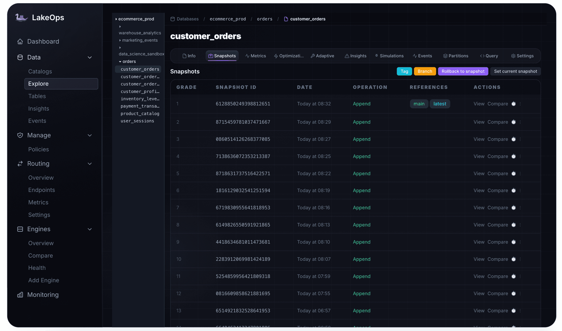
What it does: computes a health score per table from both metadata and cross-engine query telemetry, ranks the lake by severity, and makes the worst problems the ones you see first.
How it does it: LakeOps derives a health score from file count and size, manifest depth, snapshot accumulation, delete-file ratio, partition skew, and sort-order alignment with real query patterns — then classifies tables as healthy, warning, or critical across four severity tiers. Cross-engine telemetry records SELECT, FILTER, and JOIN frequency per column, which makes sort-order drift detectable and feeds key selection for compaction. It starts from a catalog connection: no agents, no pipeline changes, no manual SQL.
The shift is from per-table debugging to lake-wide triage. Instead of investigating the table someone complained about, you work a ranked list — and the tables at the top are frequently ones nobody had complained about yet. The observability page covers the scoring inputs, and the lakehouse observability guide covers what to instrument if you are building it yourself.


Governance: two kinds, and only one has an obvious home
Lakehouse governance splits cleanly in two. Conflating them is why governance conversations go in circles.
Access governance answers who may read or write what. This belongs in the catalog: RBAC in Polaris, IAM in Glue, access control in Nessie, credential vending, and Read Restrictions for row and column filtering. The catalog is the authorization boundary because it is where storage credentials originate.
Operational governance answers a different set. Which tables are maintained, and to what standard? What is the retention policy for this namespace, and can I prove it was applied? When a GDPR deletion request arrives, can I demonstrate the row is gone from every snapshot rather than merely masked? Who changed the compaction schedule on the finance tables, and when?
No catalog answers those, because they are not access questions. In most lakehouses they are answered by convention and a Git history of DAG changes — which is to say, not answered auditably. The clean formulation: access governance lives in the catalog, operational governance lives in the control plane.
The GDPR case shows why this is structural. A DELETE FROM removes a row from the current table state, but earlier snapshots still reference the data files containing it, so the data remains physically present and time-travel-readable. Actual erasure requires a sequence: delete the rows, compact to rewrite the affected files without them, expire the snapshots still referencing the originals, then remove the now-orphaned files. The order is load-bearing, and the chain has to be logged to be provable. The catalog cannot do that for you.
The control plane as the policy and audit layer
What it does: turns maintenance and retention from scripts into declarative, inherited, versioned policy, and records an auditable trail of everything that ran.
How it does it: LakeOps expresses operational governance as six policy types — expire snapshots, remove orphan files, compact data files, rewrite manifests, rewrite position delete files, and rewrite equality delete files — scoped from organization down through catalog and namespace to table, with table-level settings overriding inherited ones. New tables inherit their namespace's policy automatically. Policies support cron plus event-driven overrides, keep full version history with one-click rollback, and apply identically across Glue, Polaris, Nessie, and Gravitino.
Every operation writes an audit record: duration, files before and after, bytes reclaimed, status, and the policy that triggered it — the evidence base for SOC 2 and HIPAA, and what makes the GDPR sequence above demonstrable rather than asserted. The governance page covers the policy model, and lakehouse governance covers the broader design.


AI agents as a first-class table consumer
This is the newest layer and the one most likely to be designed for after the fact. Agents explore rather than execute known queries, so access patterns are unpredictable and scans can be accidentally enormous. They iterate quickly, so one investigation becomes dozens of queries. They need schema context to write correct SQL. And an agent has no intuition that a SELECT * against a 40 TB table is a bad idea.
Three requirements, none optional if agents have production access:
- A structured interface. Tool-shaped access with schema awareness, not a raw JDBC string and hope.
- Cost and safety limits enforced server-side. Client-side prompting is not a control. The boundary has to be in the data path.
- Layout that tolerates unpredictable filters. A table clustered for three known dashboard queries prunes badly for an agent exploring a fourth dimension. Broader clustering, current statistics, and lean metadata matter more here than in a fixed-workload architecture.
The control plane as the agent boundary
What it does: gives agents a governed, schema-aware entry point to the lakehouse with enforced guardrails, and feeds agent query behavior back into layout decisions.
How it does it: LakeOps exposes the lakehouse over the Model Context Protocol, so Claude, LangChain, and custom agents get schema-aware tools — list_catalogs, get_table_health, run_query, analyze_storage_reclaim, get_optimization_status — alongside Postgres, MySQL, and Arrow Flight SQL. Four guardrails stack, scoped per session, per team, or lake-wide: ReadOnly blocks DDL and DML, CostEstimate rejects scans above a configured size, PIIMask hashes sensitive columns before results return, and HumanApproval pauses writes pending sign-off. Every guard that fires is logged.
The loop closes here too: the columns agents filter and join on feed the same telemetry that drives compaction sort order. The agentic AI page covers the guardrail model, and connecting AI agents to Iceberg with MCP covers the integration.
The cost model, and which levers actually move it
Lakehouse spend is not dominated by storage. It is dominated by compute burned scanning data that could have been skipped, and by request overhead from too many files. Both are layout consequences. Five levers, in order of leverage:
- 1.Query-aware layout. Clustering on the columns queries actually filter reduces data scanned, which reduces compute directly. Largest lever, least used.
- 2.Storage cleanup. Expiring snapshots and removing orphans reclaims waste — 20–40% is typical on a lake that has never had it run, with reported figures reaching 56%.
- 3.Efficient compaction. Maintenance is itself a compute cost. A purpose-built engine rather than a general-purpose cluster cuts roughly 90% of the compute per terabyte compacted.
- 4.Engine routing. Sending each query to the cheapest engine that can serve it — which layout quality determines — has been measured at up to 56% lower query spend.
- 5.Autonomous operation. Engineering time not spent maintaining maintenance infrastructure compounds as table count grows.
Composite figures across production deployments: 76% lower compute cost, 12x faster queries, 51% less data scanned, 62% fewer S3 requests, and operations that scale from 50 tables to over 5,000 without proportional headcount. The cost optimization page breaks the levers down individually.
These levers are multiplicative and share one input. Better layout reduces scan cost, which reduces engine cost, which widens engine eligibility — and all of it depends on knowing what queries actually do. That shared dependency is the argument for treating operations as a layer rather than a set of chores.
A build sequence that works
Building from scratch, this order front-loads the decisions that are hard to reverse:
- 1.Storage and layout conventions. One bucket, one prefix per table, unique table locations enabled, lifecycle rules for storage class only — never deletion.
- 2.A REST catalog, deployed for real. Multi-replica, credential vending on from the start. Retrofitting short-lived credentials after every engine has a long-lived key is a migration; starting with them is a config.
- 3.One engine, one pipeline, end to end. Prove ingest, commit, and read before adding engines. Include commit-retry logic in the first pipeline.
- 4.Decide your format version deliberately. Inventory every reader first. V3 is the right default if your fleet supports it; if open-source Trino is your serving engine, plan around that.
- 5.Observability before automation. Instrument file counts, sizes, manifest depth, snapshot age, and delete ratios before writing a maintenance job. Automating against unmeasured tables is how you rewrite healthy data nightly and never touch the degraded table.
- 6.Maintenance in dependency order. Expire, compact, clean, rewrite. Get it right on one table manually before scheduling it.
- 7.Express it as policy, not scripts. Once maintenance spans more than a handful of tables, per-table scripts stop scaling.
- 8.Then add engines, routing, and agents. Additive once the foundation is sound, painful before it is.
Steps 5 through 7 are where most lakehouse projects stall — the work stops being a build and starts being an operation. That transition is what a control plane absorbs, which is why the realistic version of this sequence has one entering at step 5 rather than a later quarter.
Build it, buy a managed table service, or adopt a control plane
Three ways to cover the operational layer — they are not equivalent.
| Approach | Covers | Does not cover |
|---|---|---|
| Build with Airflow or Spark | Full control; no new vendor | You choose every threshold and sort order with no telemetry; becomes a second system |
| Managed table service (S3 Tables, Databricks) | Compaction and expiry inside that platform | Cross-catalog/engine scope; sort-order selection; tiering blind spots; operational audit |
| Control plane | Lake-wide observability, query-aware layout, adaptive maintenance, policy and audit, routing, agent guardrails | Another dependency — and not a catalog or an engine |
The honest framing of the build option: the procedures are easy and the judgment is hard. Writing a DAG that calls rewrite_data_files takes an afternoon. Knowing which of 2,000 tables to call it on today, with which sort order, at what cadence, without racing your streaming writer, and proving it helped — that does not get easier with more DAGs. Managed table services solve compaction within their own boundary, which is useful and narrower than the problem: they will not tell you your declared sort order stopped matching your query mix six months ago.
If you want the shape of a mature answer before committing, the platform overview shows how the loop is assembled, including operating modes from full autopilot through manual approval to policy-driven execution — the usual way teams stage adoption without handing over control on day one.
Where this leaves you
Four of the five layers are close to settled. Object storage is object storage. Apache Iceberg has won the table format, and V3 is the sensible floor once your readers support it. The REST catalog specification made catalog choice operational rather than architectural. Engine plurality is the normal case. You can assemble those four from good defaults and be right.
The fifth layer determines whether the first four keep working. It is usually absent from the diagram, unowned in the org chart, and discovered through a latency regression rather than a design review. Table health degrades under correct use; the remedies are known; the difficulty is continuous judgment across every table, and that judgment needs evidence from both metadata and real query behavior.
The decision to make deliberately is not which table format or which catalog. It is whether the operational layer is a first-class part of your architecture with a design and an owner, or an accumulation of scripts you will rewrite in eighteen months. A control plane is the name for treating it as the former — and on a lake of any real size, it stops being optional well before anyone declares it so.
If observability and maintenance are next on your list, looking at your own tables is a faster way to decide than reading about it. LakeOps connects to an existing catalog and reports table health across the lake without changing pipelines or moving data.