
Every production Iceberg table carries a hidden layer that determines whether an agent's query returns in 300 milliseconds or 30 seconds — and it's completely invisible to anything with only SQL access. An analyst assistant answering revenue questions in plain English. A customer support agent pulling real-time order status. An ML pipeline agent discovering features across catalogs it has never seen. These agents query Apache Iceberg tables iteratively, at high frequency, and without human review. A single user question can trigger 15–30 SQL statements — schema discovery, sampling, aggregation, drill-down, validation, and formatting — and the infrastructure they require looks nothing like what you built for dashboards and batch ETL.
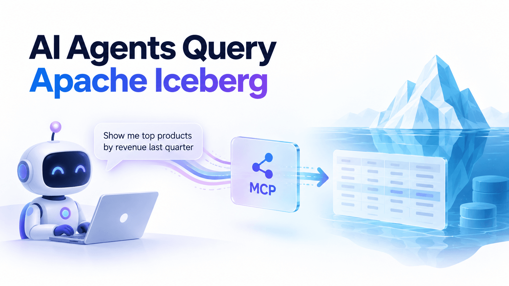
The missing piece is not a smarter model. It's a control plane — an operational layer between agents and your Iceberg tables that handles discovery, safety, routing, and optimization so you don't have to build and maintain each piece yourself. The Model Context Protocol (MCP) provides the standardized interface for agents to connect to that control plane, turning natural-language questions into governed, optimized SQL against your lakehouse.
LakeOps is an autonomous Iceberg lakehouse control plane that sits in exactly this position. It connects to your existing catalogs and query engines, then provides a single MCP server with 27 tools covering schema discovery, query execution, health monitoring, maintenance, and governance — giving every AI agent in your organization structured, governed access to your lake with zero custom integration code.
This guide walks through exactly how that works: from the moment a user types a question to the moment the agent returns an answer — and every infrastructure decision in between.
What MCP Is and Why It Matters for Data Lakehouses
The Model Context Protocol is an open standard, originally introduced by Anthropic, that defines a uniform interface for connecting AI agents to external tools and data sources. Think of it as the JDBC of the AI era — a standardized, schema-aware protocol that any compliant client can connect to without custom integration code. The protocol reached a major milestone with the 2026-07-28 specification, which made the core stateless — every request is now self-describing, servers run behind ordinary HTTP load balancers, and the sticky sessions that plagued earlier deployments are gone.
MCP defines three primitives:
- Tools — functions agents can call (e.g.,
list_catalogs,get_schema,run_query) - Prompts — pre-built workflows agents can follow
- Resources — data sources agents can read
Each tool carries a typed schema, a natural-language description, and optional annotations like readOnlyHint and destructiveHint that tell clients whether an operation reads data or modifies it. MCP clients like Cursor and Claude Desktop use these hints to show confirmation dialogs before agents execute potentially dangerous operations.
For data lakehouses specifically, MCP solves three problems that raw SQL access cannot:
- 1.Structured discovery. Agents given a generic SQL endpoint skip schema discovery more than 70% of the time — they guess table names, hallucinate columns, and produce confident-sounding wrong answers. Research from the LangChain Iceberg Toolkit study demonstrated a 33 percentage-point accuracy improvement when agents use structured discovery tools versus direct text-to-SQL, while reducing SQL injection success rates from 99% to 0%. Purpose-built MCP tools force a discovery-first workflow because the tool surface makes it the natural path.
- 1.Metadata visibility. The operational health of an Iceberg table — small-file counts, snapshot bloat, manifest fragmentation, partition skew — lives entirely in the metadata layer. SQL cannot express
needs_compactionorcompaction_score: 0.87. MCP tools can. An agent with SQL access willSELECT COUNT(*), confirm the table has records, and tell you everything looks fine — completely blind to the 940 small files inflating planning time or the 847 snapshots pinning 1.2 TB of dead storage.
- 1.Safety at the tool level. A
DROP TABLEand aSELECT 1look the same through a generic SQL endpoint. With MCP, read operations are marked read-only, destructive operations require confirmation, and permission scopes control exactly which tools each agent can call.
The Control Plane: What You Actually Need Between Agents and Iceberg
Before diving into the query workflow, it helps to understand the architecture. Agents should never hit your Iceberg tables directly. They need a control plane — an operational intelligence layer that sits between the agent and your data, providing observability, guardrails, routing, and maintenance.
Building this yourself means assembling and operating at least five independent systems: a metadata API for schema discovery, a query proxy with SQL parsing for guardrails, a routing layer with multi-engine dialect translation, a compaction pipeline with dependency-aware sequencing, and an observability backend with agent-context propagation. Each requires its own infrastructure, on-call rotation, and ongoing maintenance. Teams that go this route typically spend 3–6 months building a minimum viable version and then discover that the pieces interact in ways they didn't anticipate — compaction schedules that conflict with routing decisions, guardrails that don't account for CTE-wrapped mutations, or discovery APIs that return 8,000 tokens of raw metadata JSON where 400 would suffice.
LakeOps provides all of this as a managed control plane. It connects to your existing catalogs (AWS Glue, REST/Polaris, Nessie, Gravitino, S3 Tables) and query engines (Trino, Spark, DuckDB, Snowflake, Athena, StarRocks, Flink), then exposes the entire surface through a single MCP server. No data leaves your environment — LakeOps processes metadata only, never stores or retains it. You connect catalogs and engines in about 10 minutes, and every agent in your organization inherits structured, governed access.
Here is what the architecture looks like:
1User (natural language question)2 │3 ▼4 AI Agent (Claude, LangChain, Cursor, custom)5 │6 ▼7 MCP Server (LakeOps control plane)8 │9 ┌────┼────────────────────┐10 │ │ │11 ▼ ▼ ▼12Schema Guardrails Query Routing13Discovery (ReadOnly, (QueryFlux)14 CostEstimate, │15 PIIMask, ┌───┼───┐16 HumanApproval) │ │ │17 ▼ ▼ ▼18 Trino DuckDB Spark ...19 │ │ │20 └───┼───┘21 ▼22 Apache Iceberg Tables23 (S3 / GCS / ADLS / MinIO)The Full Query Workflow: From Natural Language to Results
Let's trace what happens when a data analyst types: "What were the top 10 products by revenue last quarter?"
Step 1: Agent Discovers the Schema via MCP
The agent doesn't guess table names. It calls MCP discovery tools to understand what data exists:
1Agent → list_catalogs()2 Returns: [{ name: "ecommerce_prod", tables: 786, size: "112.4 PB" }]3 4Agent → list_namespaces(catalog: "ecommerce_prod")5 Returns: ["orders", "products", "analytics", "payments"]6 7Agent → search_tables(catalog: "ecommerce_prod", query: "orders")8 Returns: [{ table: "customer_orders", namespace: "orders",9 size: "1.24 TB", records: 2.1B, status: "HEALTHY" }]10 11Agent → get_schema(catalog: "ecommerce_prod",12 namespace: "orders", table: "customer_orders")13 Returns: {14 columns: [15 { name: "order_id", type: "long", identifier: true },16 { name: "product_id", type: "long" },17 { name: "revenue", type: "decimal(12,2)" },18 { name: "order_date", type: "timestamp" },19 { name: "customer_id", type: "long" },20 ...21 ],22 partition_by: ["days(order_date)"],23 sort_by: ["customer_id", "order_date"]24 }This discovery-first pattern is critical. The agent now knows the exact column names, types, partition strategy, and sort order. It will not hallucinate total_sales when the column is called revenue. It knows the table is partitioned by day on order_date, which means date-filtered queries will be efficient.
Without a control plane, you'd build this yourself: a custom REST API that reads Iceberg metadata from each catalog type (Glue API, REST catalog spec, Nessie API), normalizes the output, and registers each endpoint as a tool in every agent framework you use. When you add a catalog or change a response shape, you update the API, the glue code, and the system prompt for every agent. With LakeOps, get_schema returns a compact ai_context block — schema, partition spec, sort order, and snapshot stats — in 300–500 tokens instead of the 3,000–8,000 tokens that raw Iceberg metadata JSON would consume. At 50 tool calls per agent session across hundreds of concurrent sessions, this token efficiency is the difference between agents that fit their reasoning in-context and agents that truncate critical information.
Step 2: Agent Generates SQL
With full schema context, the agent constructs accurate SQL:
1SELECT2 p.product_name,3 SUM(o.revenue) AS total_revenue4FROM ecommerce_prod.orders.customer_orders o5JOIN ecommerce_prod.products.product_catalog p6 ON o.product_id = p.product_id7WHERE o.order_date >= DATE '2026-04-01'8 AND o.order_date < DATE '2026-07-01'9GROUP BY p.product_name10ORDER BY total_revenue DESC11LIMIT 10Because the agent discovered that order_date is the partition key, it applies a tight date filter. Because it knows the column is revenue (not amount or total), the SQL is syntactically correct on the first attempt. Schema-grounded generation eliminates the most common failure mode of text-to-SQL systems: hallucinated identifiers.
Step 3: Guardrails Evaluate the Query
Before execution, the query passes through a layered guardrail pipeline. This is where giving agents raw SQL access to production data becomes dangerous — and where the control plane earns its keep.
Consider what happens without guardrails: a research agent exploring an unfamiliar dataset happily runs SELECT * FROM events on a 4 TB table, producing a result set that overflows the LLM context window and generates thousands of dollars in compute and egress costs. A coding agent asked to "clean up old data" issues DELETE statements against production tables. A customer support agent returns email addresses, SSNs, and credit card numbers in plain text — passed directly into the LLM context.
LakeOps guardrails are composable and stack per session, team, or globally:
| Guard | What It Does | Why It Matters |
|---|---|---|
| ReadOnly | Blocks DDL and DML (INSERT, DELETE, DROP, ALTER) using Rust-based SQL parsing (sqlparser-rs) — catches CTEs wrapping mutations, function calls with side effects | Prevents agents from modifying production data. Not string matching — real parsing that catches circumvention patterns |
| CostEstimate | Runs EXPLAIN before execution; rejects queries exceeding a scan threshold (e.g., 10 GB) | Stops a runaway SELECT * on a 4 TB table. Catches cartesian joins and missing-WHERE patterns before scanning a single byte |
| PIIMask | Hashes, nulls, or excludes sensitive columns (email, SSN, card numbers) before results reach the model | Keeps PII out of the LLM context window — GDPR/CCPA compliance. Three strategies: exclude (column removed entirely), hash (SHA256 pseudonym), null_out (column exists but is empty) |
| RowLimit | Injects LIMIT N when a query lacks one | Agents in reasoning loops forget to limit results. Without this, a single query can produce multi-gigabyte result sets that flood context windows |
| HumanApproval | Pauses high-stakes operations for human review via Slack/email webhook | Safety net for anything the automated guards cannot catch — DDL, queries exceeding cost thresholds, or queries touching sensitive tables |
A typical agent-facing guardrail configuration:
1groups:2 - name: analyst-agents3 guards:4 - type: read_only5 - type: row_limit6 max_rows: 50007 inject_if_missing: true8 - type: cost_estimate9 max_scanned_bytes: 10_000_000_000 # 10 GB10 - type: pii_mask11 sensitive_columns:12 "users.email": hash13 "users.ssn": exclude14 "payments.card_number": null_outGuards are evaluated sequentially — cheaper checks gate expensive ones. Every guard action is logged: what fired, what was rewritten, what was rejected — full auditability for compliance. Building this yourself means writing a SQL parsing proxy (not regex — real parsing that handles CTEs, subqueries, and engine-specific syntax), implementing EXPLAIN-based cost estimation across multiple engine dialects, building PII detection and rewriting logic, and maintaining it all as SQL standards and engine capabilities evolve.
Step 4: Query Routes to the Optimal Engine
Our analyst's query is a medium-complexity aggregation with a join. Which engine should run it?
Production Iceberg deployments rarely use a single engine. A typical setup has Trino for interactive analytics, DuckDB for lightweight lookups, Snowflake for BI, and Spark for batch ETL. The wrong routing decision at agent scale is expensive: a simple metadata lookup that costs $0.001 on DuckDB costs $0.05 on Snowflake. Across thousands of agent interactions per day, that 50× difference determines whether the workload is economically viable.
LakeOps query routing, powered by QueryFlux (an open-source Rust SQL proxy with ~0.35ms P50 overhead), makes this decision through a three-router stack:
- 1.Adaptive router — checks if this query shape has been seen before. With 20+ observations for the same parameterized template, it routes to the engine with the best P50 latency. Decision cost: 0ms (in-memory cache). Handles ~80% of agent traffic — the same
SELECT * FROM orders WHERE customer_id = ? AND status = ?that runs thousands of times per day is routed instantly based on accumulated performance data.
- 1.LLM router — for novel query shapes, uses a language model with live table statistics and engine capabilities to reason about optimal placement. The result is cached by parameterized hash, so subsequent executions of the same template skip the LLM entirely.
- 1.Semantic router — local embedding similarity against a library of known query shapes. Handles the long tail of rare patterns at ~1ms decision cost.
For our query, the adaptive router has seen this aggregation-with-join pattern before and routes it to Trino — strong at multi-table joins with 1.8s average runtime and $0.03/query cost, versus Snowflake at 2.1s and $0.08/query.
The routing is organized by routing groups — each with its own stable endpoint URL, engine pool, and guardrail stack. Agents connect to one endpoint and inherit everything automatically. You can review how routing groups work in detail on the query routing docs.
1Routing group: "Analytics"2 Endpoint: e1fa3c3c.lakeops.dev3 Engines: Trino, DuckDB4 Strategy: Latency-optimized5 Priority: HighWire compatibility supports PostgreSQL, MySQL, and Arrow Flight SQL — agents connect through standard database drivers and QueryFlux translates SQL to the target engine's dialect automatically:
1psql -h agent.lakeops.dev -U ai_agent -d ecommerce_prodThe system is self-improving: as agents run queries and execution metrics accumulate, the adaptive router builds confidence for repeated templates. New query shapes start at the LLM router, get cached, and eventually accumulate enough history to move to the adaptive router — converging toward optimal routing with zero manual configuration.
Step 5: Agent Interprets and Presents Results
The query executes on Trino, returns 10 rows, and the agent formats them into a natural-language answer:
> "The top product by revenue last quarter was the Premium Wireless Headphones at $4.2M, followed by the Ultra HD Monitor at $3.8M and the Ergonomic Keyboard at $2.1M..."
The agent can add context, compute derived metrics, compare to previous quarters, or visualize the data — all from the structured result set. The entire round trip — discovery, SQL generation, guardrail evaluation, routing, execution, and interpretation — typically completes in 2–5 seconds.
Beyond Querying: Agents That Operate the Lake
Natural-language querying is the entry point, but MCP enables agents to go far beyond reading data. With LakeOps's 27 MCP tools, agents become operational participants in your lakehouse — not just consumers.
Health Monitoring and Triage
An on-call engineer at 2 AM can ask: "Which tables need attention right now?"
1Agent → search_tables(status: "CRITICAL", sort: "tableSizeInBytes:desc")2Agent → get_table_profile(table: "raw_clickstream")3 Returns: {4 health_signals: [5 "940 small data files (avg 7 MB) — compact to reduce planning time",6 "847 snapshots pinning 1.2 TB of dead storage",7 "12 manifests fragmented to 340 MB total"8 ],9 needs_compaction: true,10 compaction_score: 0.87,11 needs_expire_snapshots: true12 }The agent produces a prioritized triage report in 15 seconds — citing concrete metrics for each table — that would take 30 minutes of dashboard clicking and manual queries. Then it calls get_table_events to see what happened recently: the last compaction ran 18 days ago, snapshot expiry has never run, and no governance policies are attached. The agent now understands not just the current state but the trajectory. Detailed observability capabilities feed into these signals automatically.
Without a control plane, this kind of triage requires an engineer to SSH into a bastion, run diagnostic queries against different engines (each with engine-specific system table syntax), manually cross-reference file counts from S3 listings, and piece together a picture of table health from fragmented signals. The agent collapses this into a few structured tool calls.
Maintenance Decisions with Sequencing
Iceberg tables degrade through four mechanisms — small-file accumulation, snapshot bloat, manifest fragmentation, and orphan files — and the fix order matters. Snapshot expiry must precede orphan cleanup (expiry marks files as unreferenced; cleanup deletes them). Compaction must precede manifest rewriting (compaction changes the file set; new manifests are already optimal). Running them independently as disconnected cron jobs produces conflicts and redundant work.
LakeOps encodes this sequencing logic into the tool layer so agents don't need to know the dependency graph:
1Agent → analyze_table_maintenance(table: "raw_clickstream")2 Returns: {3 recommendations: [4 "1. Enable ADAPTIVE_MAINTENANCE for continuous compaction",5 "2. Set snapshot retention to 10, 7-day age window",6 "3. Defer orphan cleanup until after expiry is established"7 ],8 rationale: "Compaction first — 940 small files inflate planning time.9 Expiry second — 847 snapshots pin 1.2 TB.10 Orphan cleanup after — requires expired snapshots to be useful."11 }This is operational knowledge encoded directly into the tool layer. Instead of expecting every agent (or every engineer writing agent prompts) to independently know that snapshot expiry must precede orphan cleanup, the tools embed that logic and return actionable, sequenced guidance.
Governance Policy Management
If the engineer approves, a write-scoped agent can create policies directly:
1Agent → create_policy(2 type: "ADAPTIVE_MAINTENANCE",3 catalog: "marketing_events",4 namespace: "analytics",5 table: "raw_clickstream",6 config: { target_file_size: "512MB", snapshot_retention: 10 }7)The destructiveHint annotation on execute_policy means MCP clients prompt for human confirmation before triggering execution — the agent proposes, the human approves. Other write tools like create_policy and update_policy define or update policy definitions but don't run maintenance directly.
Why Tables Must Be Healthy Before Agents Can Query Them
Here is a detail most guides skip: routing and MCP sophistication cannot compensate for unhealthy tables. An agent hitting a table with 47,000 small files will timeout regardless of how smart the routing is. Agent query P95 latency on uncompacted tables runs 50+ seconds due to S3 GET amplification and manifest listing overhead. The same query on a compacted, sorted table returns in under 1 second. An agent that gets slow responses issues more queries — retries, timeouts, and recovery queries that compound the load. A slow lake makes the agent problem worse, not just slower.
This is where the control plane pays for itself. LakeOps runs a Rust-based compaction engine with Apache DataFusion that continuously optimizes tables for the queries actually hitting them — including agent queries:
- Query-aware compaction — analyzes which columns agents filter, join, and group on, then physically re-sorts data to match. Engines skip entire file groups via min/max pruning. If agents predominantly filter on
event_timestampanduser_id, data is re-sorted on those columns so Parquet row group statistics enable predicate pushdown — eliminating irrelevant row groups before any S3 read. - 95% faster than Spark — benchmarks show 221 seconds (LakeOps) vs. 1,612 seconds (Spark) vs. 6,300 seconds (S3 Tables) on identical 200 GB datasets, at $5/TB vs. Spark's $50/TB.
- Layout simulation on branches — LakeOps tests layout changes on Iceberg branches before they touch production. Compare scan reduction, file count, and estimated speedup side by side, then apply the winning change with one action. No guesswork, no rewrite risk.
- Self-improving — sort orders adapt as agent query patterns evolve. The lake gets faster the more agents use it.
The compound effect is powerful: as storage optimizes for agent access patterns, more engines become viable for each query shape. A query that required Trino pre-compaction might run on DuckDB afterward — cheaper and faster. Routing options expand, which generates more performance data, which further improves both routing and compaction decisions.
Workload Profiles: Tuning Guardrails and Routing per Agent Type
Different agents produce fundamentally different workload shapes. Configuring per workload type — rather than treating all agent traffic as homogeneous — is where the largest gains materialize.
| Agent Type | Guard Stack | Routing Strategy | Latency Target |
|---|---|---|---|
| BI assistant | ReadOnly + RowLimit(1000) + CostEstimate | Latency (DuckDB, Trino) | < 500ms p95 |
| Customer chatbot | ReadOnly + RowLimit(100) + PIIMask + CostEstimate | Latency (DuckDB, cached) | < 500ms p95 |
| Data exploration | ReadOnly + RowLimit(5000) + PIIMask | Cost (DuckDB metadata, Trino scans) | < 10s p95 |
| ETL orchestrator | HumanApproval + CostEstimate | Throughput (Spark, Athena) | < 5s p95 |
| ML feature agent | ReadOnly + RowLimit(500) + CostEstimate(1GB) | Latency (DuckDB, StarRocks) | < 200ms p95 |
Each profile maps to a routing group with its own stable endpoint, engine pool, and guardrail stack. An interactive chatbot agent connects to the low-latency pool; an ETL agent connects to the compute-optimized pool. Both inherit their full policy stack automatically. Read the full agentic AI architecture for deeper configuration guidance.
Setting Up MCP Access: A 10-Minute Walkthrough
Connecting an AI agent to your Iceberg lakehouse through LakeOps MCP takes two steps.
1. Create a Scoped API Key
In the LakeOps dashboard, navigate to Organization → API Keys. Create a key with the scopes your agent needs:
| Scope | Grants |
|---|---|
read | All discovery and analysis tools — schema inspection, health monitoring, maintenance signals |
write | Policy management — create, update, enable, disable, execute policies |
query:read | Ad-hoc SQL queries through the routing and guardrail pipeline |
Start with read + query:read. Add write when you are ready for agent-managed governance. Scopes are independent — write does not implicitly include read, so agents that discover data and then manage policies need both.
2. Configure Your MCP Client
For Cursor, add to .cursor/mcp.json:
1{2 "mcpServers": {3 "lakeops-us-east-1": {4 "url": "https://api.lakeops.dev/mcp",5 "headers": {6 "Authorization": "Bearer <your-api-key>"7 }8 }9 }10}For Claude Desktop, add the same block to claude_desktop_config.json. For LangChain, LlamaIndex, or custom agents, any MCP-compatible client connects the same way.
Multi-region deployments add one server entry per region (lakeops-us-east-1, lakeops-eu-west-1, lakeops-ap-south-1). API keys are region-scoped — match the key to the endpoint. A region mismatch is the most common setup mistake — a key for a Mumbai org against the US endpoint returns empty catalogs with no obvious error.
That's it. Every connected agent auto-discovers all 27 tools and inherits the guardrail stack of its endpoint. No glue code, no prompt engineering, no per-agent maintenance.
The Closed-Loop System
The five components — MCP connectivity, guardrails, multi-engine routing, self-optimizing storage, and observability — are not independent tools. They form a closed loop that improves autonomously:
- 1.Agents connect via MCP — schema-aware tools auto-discovered, stable endpoints per workload, structured access with zero integration code.
- 2.Guardrails enforce safety — every query passes through composable guards before execution. Every guard action is logged with agent ID, conversation context, and the original query — full auditability for SOC 2, GDPR, and CCPA.
- 3.Routing optimizes cost and latency — each query dispatches to the cheapest viable engine. The adaptive router handles ~80% of traffic at 0ms decision cost.
- 4.Storage self-optimizes — compaction, manifests, snapshots, and cleanup run continuously as a coordinated pipeline, informed by agent query telemetry. Agent access patterns feed back into sort-order decisions. Hot tables get elevated compaction priority.
- 5.Observability closes the loop — per-agent metrics feed back into routing decisions, compaction priorities, and guardrail tuning. Given a
conversation_id, you can reconstruct the entire sequence of SQL queries an agent issued during a single interaction — turning query history into an agent reasoning debugger.
The measurable outcomes on production deployments: agent query P95 drops from 5–10 seconds to under 500ms. Per-query compute cost drops 65% through intelligent routing. Guardrails prevent an average of 3.2 petabyte-scale scans per day. And the system improves autonomously — no manual query log analysis, no sort-order tuning by hand, no routing rule maintenance.
Getting Started
Three steps, in order:
Step 1: Get your tables healthy. An agent hitting a table with 200,000+ small files will timeout regardless of how sophisticated the MCP layer is. Enable continuous compaction, snapshot expiration, and manifest consolidation first. This is a prerequisite, not an optimization — uncompacted tables pay a 5–10× latency penalty that no amount of routing can compensate for.
Step 2: Deploy guardrails before the first agent query. Start with ReadOnly and RowLimit on every agent session. Add CostEstimate with a conservative threshold (10 GB). The cost of deploying guards too early is zero. The cost of deploying them too late is one bad query that scans your entire lake.
Step 3: Enable routing and observability. Connect your engines, configure routing groups per agent workload type, and enable per-agent cost attribution. Within a week you will have the data to understand which agents are expensive, which tables are slow, and where to optimize next.
LakeOps connects to your existing catalogs and object storage in about 10 minutes. No agents to install, no data to move, no pipelines to modify. Your data stays in your account. Supported catalogs include AWS Glue, REST (Polaris, Gravitino, Nessie, Lakekeeper), and S3 Tables. Read more about the full platform architecture and explore the Iceberg with AI agents deep dive for production-level implementation details.
The lakehouse stack now has three standard interfaces: object storage for data files, REST catalogs for query engines, and MCP for AI agents. The agents that succeed in production will not be the ones with the most elaborate system prompts — they will be the ones connected to structured, scoped, purpose-built tools backed by a control plane that keeps the underlying data fast, safe, and governed.